Prepare for your next AI engineer role with this comprehensive guide — from foundational ML theory and transformer architecture all the way to LLM fine-tuning, RAG pipelines, production serving, and responsible AI. Questions are organised by difficulty so you can track your progress at every stage.
An AI Engineer sits at the intersection of software engineering and machine learning. Unlike a research scientist, the AI Engineer's primary responsibility is to build, deploy, and maintain AI-powered systems — writing the glue code between a foundation model and a production product. In 2026 that means:
This guide covers all 25 questions that appear with the highest frequency across interviews at AI-native companies, Big Tech, and top startups — based on patterns across the 2025–2026 hiring cycle.
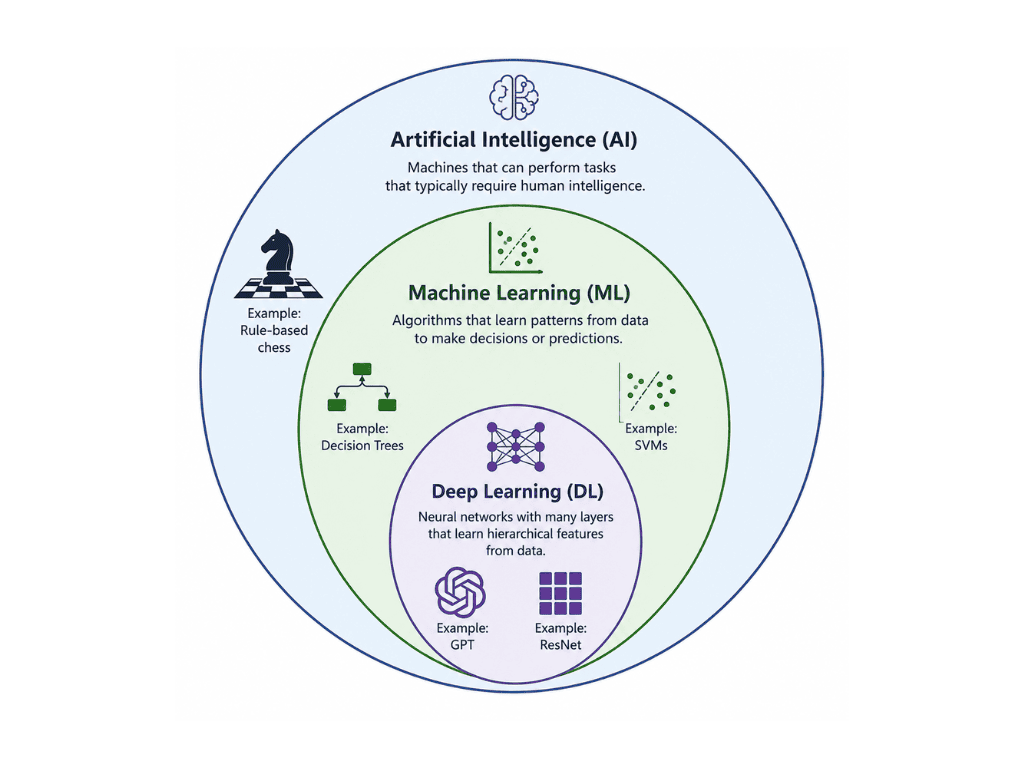
These terms represent hierarchical fields of study, where each is a subset of the one before it.
Key Definitions:
- Artificial Intelligence (AI): The broad science of mimicking human abilities (logic, reasoning, perception) through machines.
- Machine Learning (ML): A subset of AI focused on algorithms that learn patterns from data rather than following static rules.
- Deep Learning (DL): A subset of ML that uses multi-layered neural networks to learn complex, hierarchical representations.
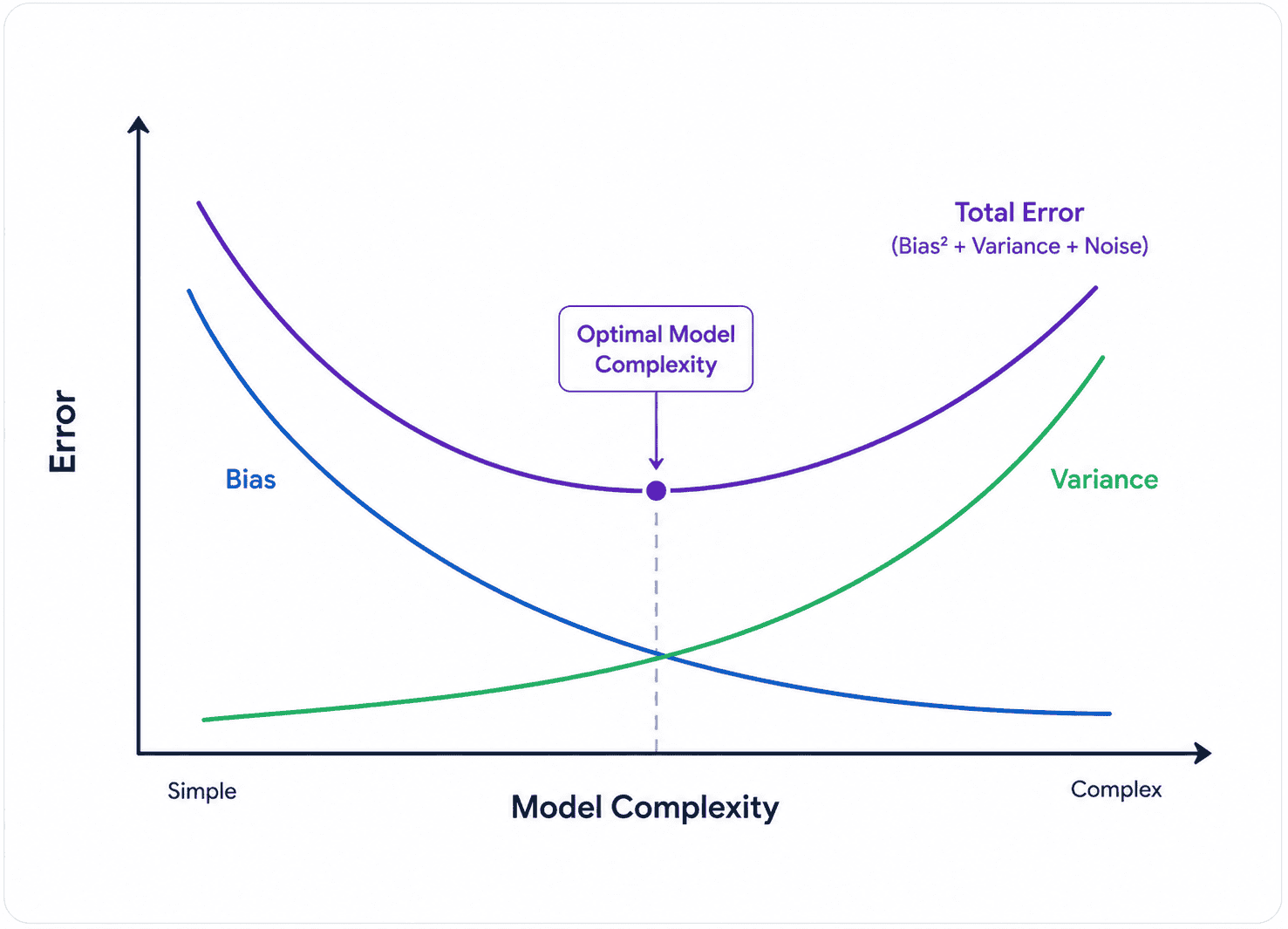
The bias-variance tradeoff is the central challenge in supervised learning: balancing model simplicity (to avoid underfitting) with model complexity (to avoid overfitting).
Components:
- Bias: Error from overly simplistic assumptions. High bias leads to underfitting (the model misses relevant patterns).
- Variance: Error from high sensitivity to small fluctuations in the training set. High variance leads to overfitting (the model interprets noise as signal).
- The Goal: To minimize the 'Total Error' by finding the optimal point where bias and variance reach a joint minimum.
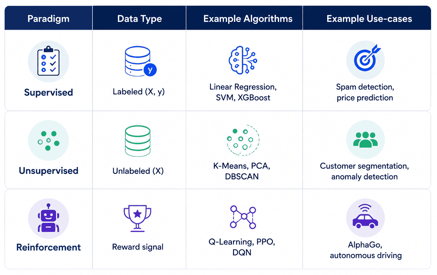
These are the three primary paradigms of machine learning, categorized by how the model receives a signal to learn.
Main Paradigms:
- Supervised: Learning with a teacher. The model is given labeled data (X, y) and learns to map inputs to specific targets (e.g., Image Classification).
- Unsupervised: Learning without labels. The model searches for hidden structures or clusters in raw data (e.g., Customer Segmentation).
- Reinforcement: Learning through interaction. An agent gains 'rewards' or 'penalties' by taking actions in an environment (e.g., Game-playing AI).
These metrics provide a more nuanced view of model performance than simple accuracy, especially when dealing with imbalanced datasets.
Core Metrics:
- Precision: 'Of all the positive predictions we made, how many were correct?' (TP / TP + FP).
- Recall: 'Of all the actual positives that exist, how many did we successfully find?' (TP / TP + FN).
- F1-Score: The harmonic mean of precision and recall. It's useful when you want to achieve a balance between the two.
# Confusion matrix components
# TP = True Positive,  FP = False Positive
# TN = True Negative,  FN = False Negative

precision = TP / (TP + FP)   # Quality of positive predictions
recall    = TP / (TP + FN)   # Coverage of actual positives
f1        = 2 * (precision * recall) / (precision + recall)
accuracy  = (TP + TN) / (TP + TN + FP + FN)  # misleading if imbalanced

# Example: fraud detection on 10,000 transactions (50 are fraud)
# A "predict nothing is fraud" classifier gets 99.5% accuracy — but recall = 0
# → Use precision/recall, ROC-AUC, or PR-AUC instead

from sklearn.metrics import classification_report
print(classification_report(y_true, y_pred))Overfitting happens when a model learns the training data 'too well'—including its noise and outliers—resulting in poor performance on new, unseen data.
How to Prevent It:
- Regularization: Penalizing large weights (L1/L2).
- Dropout: Randomly deactivating neurons during training in neural networks.
- Early Stopping: Stopping training once the validation error starts to rise.
- More Data: Increasing the size and diversity of the dataset helps the model generalize better.
import torch.nn as nn

class RegularizedNet(nn.Module):
    def __init__(self):
        super().__init__()
        self.fc1 = nn.Linear(256, 128)
        self.dropout = nn.Dropout(p=0.3)   # drop 30% of neurons randomly
        self.bn     = nn.BatchNorm1d(128)  # batch normalisation stabilises training
        self.fc2 = nn.Linear(128, 10)

    def forward(self, x):
        x = torch.relu(self.fc1(x))
        x = self.dropout(x)                # applied only during training
        x = self.bn(x)
        return self.fc2(x)

# L2 regularisation via weight_decay in the optimizer
optimizer = torch.optim.Adam(model.parameters(), lr=1e-3, weight_decay=1e-4)

# Early stopping — stop when val loss stops improving
best_val_loss = float('inf')
patience = 5
for epoch in range(100):
    train_loss = train_one_epoch(model, train_loader)
    val_loss   = evaluate(model, val_loader)
    if val_loss < best_val_loss:
        best_val_loss = val_loss; patience_counter = 0
        torch.save(model.state_dict(), 'best_model.pt')
    else:
        patience_counter += 1
        if patience_counter >= patience:
break # early stopCross-validation is a robust method for estimating how well a model will generalize to an independent dataset.
Key Benefits:
- Reliability: Instead of relying on one train/test split, it averages performance across multiple 'folds' (K-Fold).
- Efficiency: It allows you to use your entire dataset for both training and validation over multiple iterations.
- Hyperparameter Tuning: It prevents overfitting to a specific validation set during the tuning process.
from sklearn.model_selection import KFold, cross_val_score
from sklearn.ensemble import RandomForestClassifier

X, y = load_dataset()   # your features and labels
model = RandomForestClassifier(n_estimators=100)

# 5-fold cross-validation
kf    = KFold(n_splits=5, shuffle=True, random_state=42)
scores = cross_val_score(model, X, y, cv=kf, scoring='f1_macro')

print(f"CV F1 scores: {scores}")
print(f"Mean: {scores.mean():.3f} ± {scores.std():.3f}")

# Stratified K-Fold — preserves class balance in each fold
from sklearn.model_selection import StratifiedKFold
skf = StratifiedKFold(n_splits=5, shuffle=True, random_state=42)
scores = cross_val_score(model, X, y, cv=skf, scoring='roc_auc')

# Leave-one-out CV (LOOCV) — for very small datasets
from sklearn.model_selection import LeaveOneOut
loo_scores = cross_val_score(model, X, y, cv=LeaveOneOut())Gradient descent is the optimization algorithm used to minimize the cost function by iteratively updating model parameters.
Main Variants:
- Batch Gradient Descent: Computes the gradient for the entire dataset at once. Stable but very slow.
- Stochastic Gradient Descent (SGD): Computes the gradient for one single example. Fast but very noisy.
- Mini-Batch Gradient Descent: The industry standard. Computes gradients on small batches (e.g., 32 or 64 samples), balancing speed and stability.
import numpy as np

# -- Batch Gradient Descent --
for epoch in range(epochs):
    grad = compute_gradient(X_train, y_train, weights)   # entire dataset
    weights -= lr * grad

# -- Stochastic GD --
for epoch in range(epochs):
    for x_i, y_i in zip(X_train, y_train):              # one sample
        grad = compute_gradient(x_i, y_i, weights)
        weights -= lr * grad

# -- Mini-Batch SGD (standard) --
batch_size = 64
for epoch in range(epochs):
    for i in range(0, len(X_train), batch_size):
        x_batch = X_train[i : i + batch_size]
        y_batch = y_train[i : i + batch_size]
        grad = compute_gradient(x_batch, y_batch, weights)
        weights -= lr * grad

# PyTorch DataLoader handles mini-batch shuffling automatically:
loader = torch.utils.data.DataLoader(dataset, batch_size=64, shuffle=True)In deep neural networks, gradients are propagated backward. If these gradients are very small (<1), they shrink exponentially as they reach earlier layers, effectively stopping those layers from learning.
Common Solutions:
- Activation Functions: Using ReLU instead of Sigmoid/Tanh.
- Residual Connections: Skip connections (ResNets) allow gradients to flow directly.
- Batch Normalization: Stabilizes the distribution of activations.
- Better Initialization: Using He or Xavier initialization to keep weights in a healthy range.
import torch.nn as nn

# PROBLEM: Sigmoid activations collapse gradients
# d/dx sigmoid(x) ≈ 0.25 max — multiply across 20 layers → ~0.25^20 ≈ 9e-13

# SOLUTION 1: ReLU — gradient is 1 for positive inputs (no shrinkage)
nn.ReLU()

# SOLUTION 2: He initialisation — scales weights by sqrt(2/fan_in)
nn.init.kaiming_uniform_(layer.weight, nonlinearity='relu')

# SOLUTION 3: Residual connections (skip-connections)
class ResBlock(nn.Module):
    def __init__(self, dim):
        super().__init__()
        self.block = nn.Sequential(
            nn.Linear(dim, dim), nn.ReLU(),
            nn.Linear(dim, dim)
        )
    def forward(self, x):
        return x + self.block(x)  # gradient flows directly through x: d/dx = 1

# SOLUTION 4: Gradient clipping — prevent explosions, keep stability
torch.nn.utils.clip_grad_norm_(model.parameters(), max_norm=1.0)

# SOLUTION 5: Batch Normalisation — re-centers activations each layer
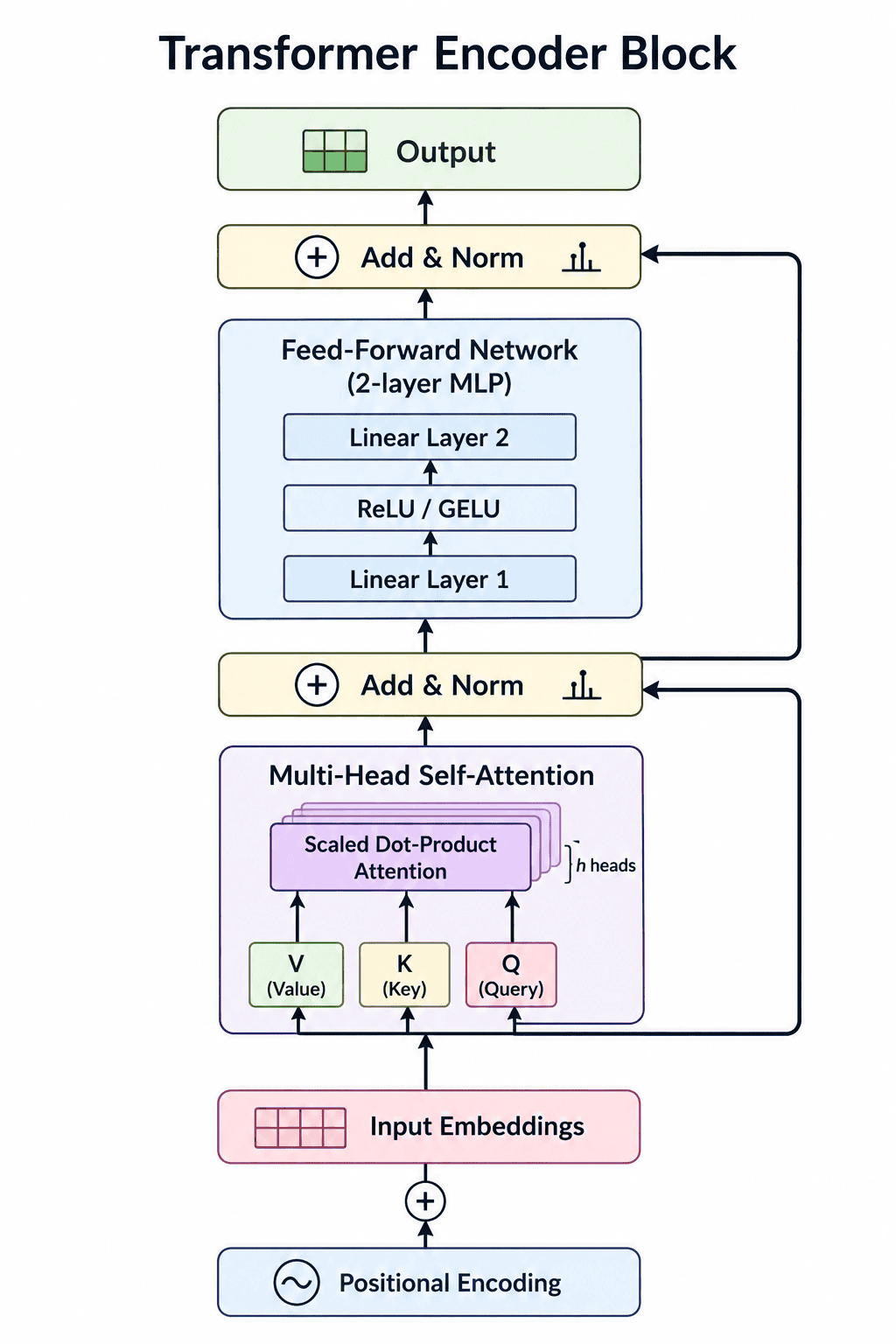
nn.BatchNorm1d(hidden_dim)The Transformer architecture, introduced in 'Attention Is All You Need', revolutionized NLP by replacing recurrent layers with a parallelizable attention-based structure.
Key Mechanisms:
- Self-Attention: Allows the model to weigh the importance of different tokens in a sequence relative to a specific token. Each token is projected into Query (Q), Key (K), and Value (V) vectors.
- Multi-Head Attention: Runs multiple attention processes in parallel, allowing the model to focus on different parts of the input simultaneously.
- Positional Encoding: Since Transformers don't process data sequentially, positional encodings are added to embeddings to provide information about a token's location.
import torch
import torch.nn.functional as F

def scaled_dot_product_attention(Q, K, V, mask=None):
    """
    Q: (batch, heads, seq_len, d_k)
    K: (batch, heads, seq_len, d_k)
    V: (batch, heads, seq_len, d_v)
    """
    d_k = Q.size(-1)
    # 1. Compute raw attention scores
    scores = Q @ K.transpose(-2, -1) / (d_k ** 0.5)  # (batch, heads, seq, seq)

    # 2. Apply optional causal/padding mask
    if mask is not None:
        scores = scores.masked_fill(mask == 0, float('-inf'))

    # 3. Softmax over key dimension → attention weights
    attn_weights = F.softmax(scores, dim=-1)           # sums to 1 per query

    # 4. Weighted sum of values
    return attn_weights @ V                            # (batch, heads, seq, d_v)

# Multi-head: run H parallel attention heads, concat and project
import torch.nn as nn
mha = nn.MultiheadAttention(embed_dim=512, num_heads=8, batch_first=True)
# In PyTorch:
output, attn_weights = mha(query=x, key=x, value=x) # self-attentionTokenization is the process of converting raw text into numerical representations (tokens) that a machine learning model can process.
Modern Approaches:
- Byte-Pair Encoding (BPE): The most common method for LLMs (like GPT). It starts with characters and iteratively merges the most frequent pairs into subword tokens.
- SentencePiece: A language-independent subword tokenizer that treats the input as a raw stream of characters, including whitespace.
- Efficiency: Subword tokenization balances the granularity of character-level models with the efficiency of word-level models, avoiding 'Out of Vocabulary' (OOV) issues.
# Using OpenAI's tiktoken (used by GPT-3.5, GPT-4)
import tiktoken

enc = tiktoken.get_encoding("cl100k_base")   # encoding used by GPT-4
text = "Hello, AI Engineer!"
tokens = enc.encode(text)
print(tokens)          # [9906, 11, 15592, 17855, 0]  (IDs, not text)
print(len(tokens))     # 5 tokens for 20 chars

# Decode back
print(enc.decode(tokens))  # "Hello, AI Engineer!"

# Show individual token strings
for tok in tokens:
    print(repr(enc.decode([tok])))  # 'Hello', ',', ' AI', ' Engineer', '!'

# Hugging Face Tokenizers — SentencePiece / BPE
from transformers import AutoTokenizer
tok = AutoTokenizer.from_pretrained("meta-llama/Llama-3-8B")
ids = tok.encode("Hello, AI Engineer!")
print(tok.convert_ids_to_tokens(ids))   # shows subword pieces

# Key insight: context window is in TOKENS, not words!
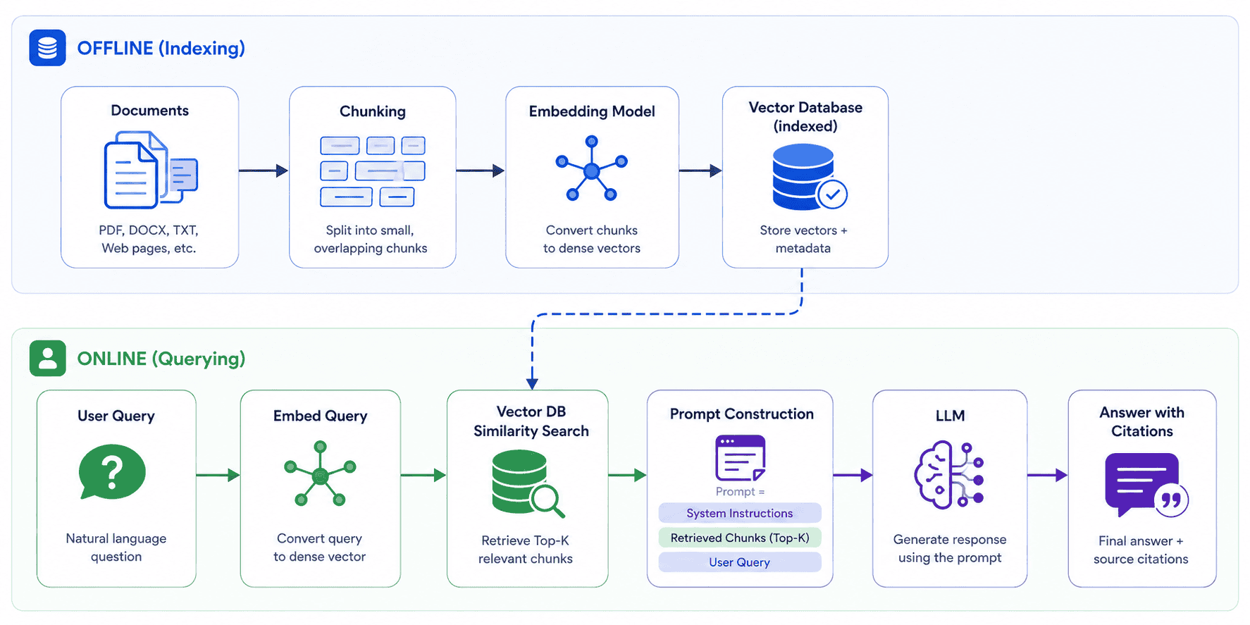
# "antidisestablishmentarianism" = 1 word ≈ 5–7 tokensRetrieval-Augmented Generation (RAG) combines the generative power of LLMs with the factual accuracy of external data stores.
The RAG Workflow:
- Retrieval: When a query is received, the system searches a vector database for relevant document chunks.
- Augmentation: These retrieved chunks are added to the user's prompt as additional context.
- Generation: The LLM generates a response based on both its pre-trained knowledge and the provided context, reducing hallucinations.
from langchain_openai import OpenAIEmbeddings, ChatOpenAI
from langchain_community.vectorstores import Chroma
from langchain.text_splitter import RecursiveCharacterTextSplitter
from langchain.chains import RetrievalQA

# ── INDEXING (run once or on document updates) ──────────────────────
from langchain_community.document_loaders import PyPDFLoader
docs   = PyPDFLoader("docs/company_handbook.pdf").load()
chunks = RecursiveCharacterTextSplitter(
            chunk_size=500, chunk_overlap=50
         ).split_documents(docs)

embedder = OpenAIEmbeddings(model="text-embedding-3-small")
db       = Chroma.from_documents(chunks, embedder, persist_directory="./db")

# ── RETRIEVAL + GENERATION (at query time) ──────────────────────────
qa_chain = RetrievalQA.from_chain_type(
    llm=ChatOpenAI(model="gpt-4o"),
    retriever=db.as_retriever(search_kwargs={"k": 5}),  # top-5 chunks
    return_source_documents=True,
)
result = qa_chain.invoke({"query": "What is our parental leave policy?"})
print(result["result"])
print(result["source_documents"]) # includes page referencesThese are different strategies for adapting an LLM to specific tasks or domains, each with varying levels of resource intensity.
Comparison:
- Prompting: Changing the input instructions without altering model weights. Lowest cost.
- In-Context Learning (ICL): Providing examples within the prompt (Few-Shot) to guide the model's behavior.
- Fine-Tuning: Updating the model's parameters on a specialized dataset. Highest cost but most effective for deep domain expertise.
- PEFT/LoRA: Parameter-Efficient Fine-Tuning which updates only a tiny fraction of weights.
# ── FEW-SHOT PROMPTING (In-Context Learning) ──────────────────────
prompt = """
Classify the sentiment.

Text: "The food was amazing!" → Positive
Text: "Terrible experience."  → Negative
Text: "It was okay I guess."  → Neutral

Text: "I absolutely loved the staff." →
"""
# Model completes: "Positive"

# ── PARAMETER-EFFICIENT FINE-TUNING (LoRA) ────────────────────────
from peft import LoraConfig, get_peft_model, TaskType
from transformers import AutoModelForCausalLM

model = AutoModelForCausalLM.from_pretrained("meta-llama/Llama-3-8B")

lora_config = LoraConfig(
    task_type=TaskType.CAUSAL_LM,
    r=16,               # rank of the low-rank matrices
    lora_alpha=32,      # scaling factor
    target_modules=["q_proj", "v_proj"],  # inject into attention layers
    lora_dropout=0.05,
    bias="none",
)
peft_model = get_peft_model(model, lora_config)
peft_model.print_trainable_parameters()
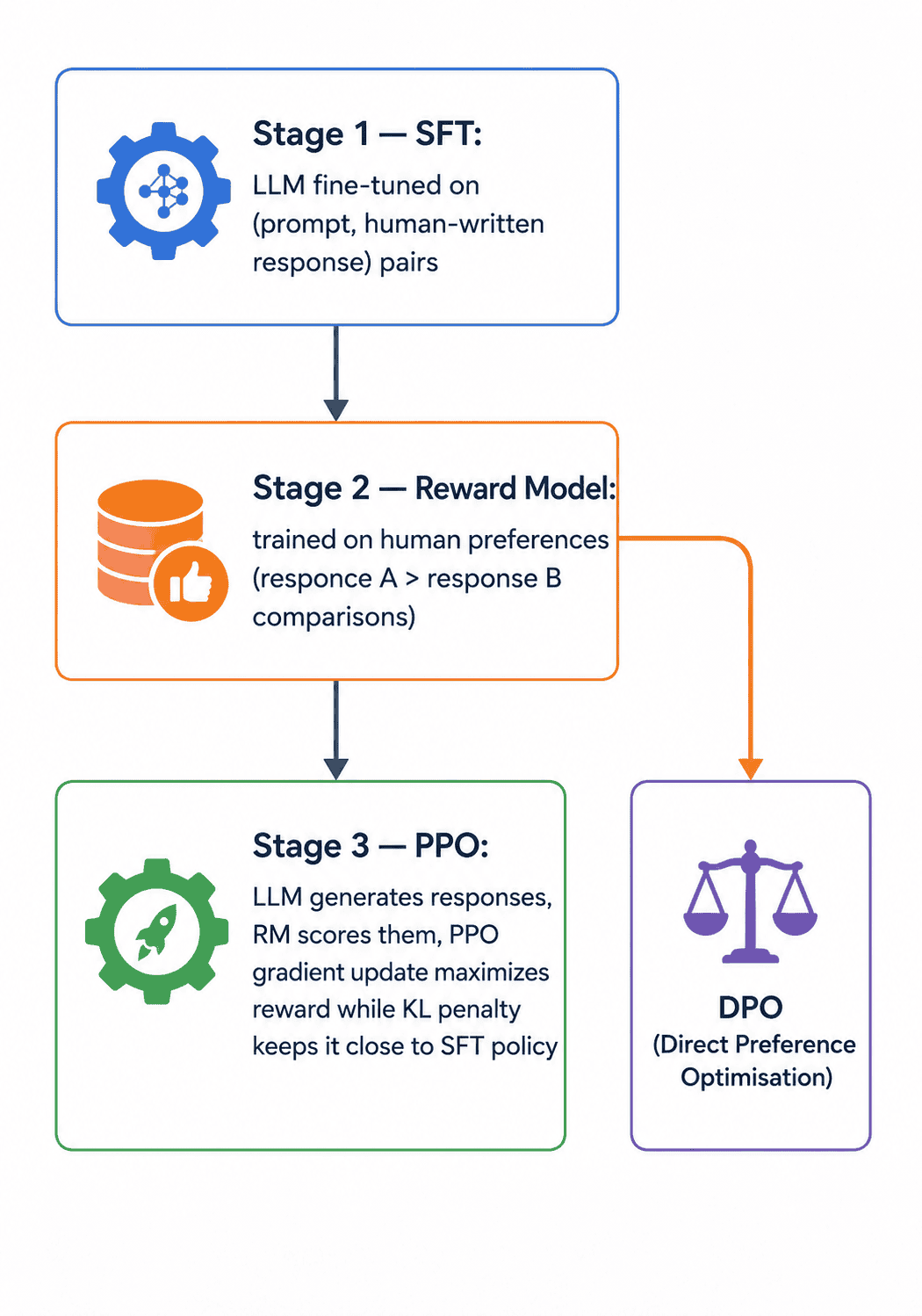
# trainable params: 4,194,304 || all params: 8,034,770,944 → 0.052%Reinforcement Learning from Human Feedback (RLHF) is the process used to 'align' models like ChatGPT so they are helpful, honest, and harmless.
Three Major Stages:
1. Supervised Fine-Tuning (SFT): Fine-tuning a pre-trained model on high-quality human-written samples.
2. Reward Modeling: Training a separate 'Reward Model' based on human preferences (ranking different outputs).
3. PPO Fine-Tuning: Using Reinforcement Learning (PPO) to optimize the model to maximize the reward from the Reward Model.
# RLHF in pseudocode (Concept — for production use trl library)
# Stage 1: SFT
model = GPT_SFT.train(prompt_response_pairs)   # supervised fine-tune

# Stage 2: Reward Model
# Human labellers rank: response_A > response_B for a given prompt
reward_model = RewardModel.train(
    chosen=response_A,
    rejected=response_B
)  # learns to assign higher score to preferred responses

# Stage 3: PPO Loop
for prompt in prompts:
    response = model.generate(prompt)                  # actor generates
    reward   = reward_model.score(prompt, response)    # critic scores
    kl_penalty = kl_divergence(model, reference_sft_model)  # stay close
    loss = -reward + beta * kl_penalty                 # PPO objective
    loss.backward()                                    # update actor

# Modern alternative: DPO (no RL loop needed)
from trl import DPOTrainer
dpo = DPOTrainer(model, ref_model, beta=0.1,
                 tokenizer=tok, train_dataset=pref_data)
dpo.train()Vector databases are designed to store and search through high-dimensional data (embeddings) efficiently using similarity metrics instead of exact matches.
How it works:
- Embeddings: Text or images are converted into long lists of numbers that represent their 'meaning'.
- Similarity Metrics: Methods like Cosine Similarity or Euclidean Distance calculate how 'close' two vectors are.
- Indexing: Advanced algorithms like HNSW or FAISS allow for Approximate Nearest Neighbor (ANN) search across millions of records in milliseconds.
import numpy as np

# -- Similarity metrics (most vector DBs support all three) --
def cosine_similarity(a, b):
    return np.dot(a, b) / (np.linalg.norm(a) * np.linalg.norm(b))
    # Range: [-1, 1]. Most common for embeddings — normalises for magnitude.

def dot_product(a, b):
    return np.dot(a, b)
    # Sensitive to magnitude — preferred when embeddings are L2-normalised.

def euclidean_distance(a, b):
    return np.linalg.norm(a - b)
    # Geometric distance — lower = more similar.

# -- Using FAISS for fast ANN search (runs locally, no API needed) --
import faiss

d     = 1536                          # embedding dimension (text-embedding-3-small)
index = faiss.IndexFlatL2(d)          # exact L2 search
index.add(stored_embeddings)          # add your vectors (np.float32)

query_vec = embed("What is our leave policy?")  # shape: (1, 1536)
D, I = index.search(query_vec, k=5)   # D=distances, I=indices
# I contains the row indices of the 5 most similar chunks

# For production scale use IndexHNSWFlat (fast, approximate)
index_hnsw = faiss.IndexHNSWFlat(d, 32)   # M=32 graph connections
index_hnsw.add(stored_embeddings)Prompt engineering is the art of crafting inputs to get the most reliable and accurate outputs from an LLM without changing the model itself.
Top Techniques:
- Chain of Thought (CoT): Asking the model to 'think step by step' to solve complex reasoning problems.
- Few-Shot Prompting: Providing a few examples of inputs and desired outputs within the prompt.
- Structured Output: Forcing the model to return data in a specific format like JSON or Markdown.
- ReAct: A framework where the model alternates between reasoning and taking actions using external tools.
# ── CHAIN-OF-THOUGHT (CoT) ─────────────────────────────────────────
zero_shot_cot = """
Solve step by step:
A store has 24 apples. They sell 1/3 in the morning and 1/4 of the
remaining in the afternoon. How many remain?

Let's think step by step:
"""
# Model reasons through: 24 → sold 8 morning → 16 remain → sold 4 afternoon → 12

# ── FEW-SHOT with STRUCTURED OUTPUT ────────────────────────────────
system_prompt = """
You are a JSON API. Extract entities from user text.
Return strictly valid JSON matching this schema:
{ "name": string, "email": string | null, "company": string | null }

# Examples:
User: "Contact John Smith at j.smith@acme.com, works at Acme Corp"
Assistant: {"name":"John Smith","email":"j.smith@acme.com","company":"Acme Corp"}

User: "Email from Sarah (no email listed), freelancer"
Assistant: {"name":"Sarah","email":null,"company":null}
"""

# ── REACT AGENT PATTERN ─────────────────────────────────────────────
react_prompt = """
You have access to: [search_web(query), calculator(expr), set_reminder(time, text)]

Thought: I need to find the current USD/EUR rate.
Action: search_web("USD EUR exchange rate today")
Observation: 1 USD = 0.92 EUR as of June 24 2026.
Thought: Now I can answer.
Answer: Today's USD to EUR rate is 0.92.
"""AI agents are systems where the LLM is given the autonomy to use external tools to complete a complex objective.
Mechanics:
- Tool Definition: The agent is given a list of available 'tools' (APIs, calculators, search engines) described via JSON schemas.
- Function Calling: The model decides which tool to use and generates the necessary arguments.
- Execution Loop: The system executes the tool, feeds the result back to the LLM, and the model decides the next step based on that new information.
import openai, json

client = openai.OpenAI()

# Define available tools as JSON schemas
tools = [
    {
        "type": "function",
        "function": {
            "name": "get_weather",
            "description": "Get the current weather for a city",
            "parameters": {
                "type": "object",
                "properties": {
                    "city": {"type": "string", "description": "City name"},
                    "unit": {"type": "string", "enum": ["celsius", "fahrenheit"]},
                },
                "required": ["city"],
            },
        }
    }
]

messages = [{"role": "user", "content": "What's the weather in Tokyo?"}]
response = client.chat.completions.create(
    model="gpt-4o", messages=messages, tools=tools, tool_choice="auto"
)

msg = response.choices[0].message
if msg.tool_calls:
    call = msg.tool_calls[0]
    args = json.loads(call.function.arguments)  # {"city": "Tokyo"}

    # Execute the actual function
    weather_result = get_weather(**args)        # your real implementation

    # Feed result back into the conversation
    messages.append(msg)
    messages.append({
        "role": "tool",
        "tool_call_id": call.id,
        "content": json.dumps(weather_result)
    })
    final = client.chat.completions.create(model="gpt-4o", messages=messages)
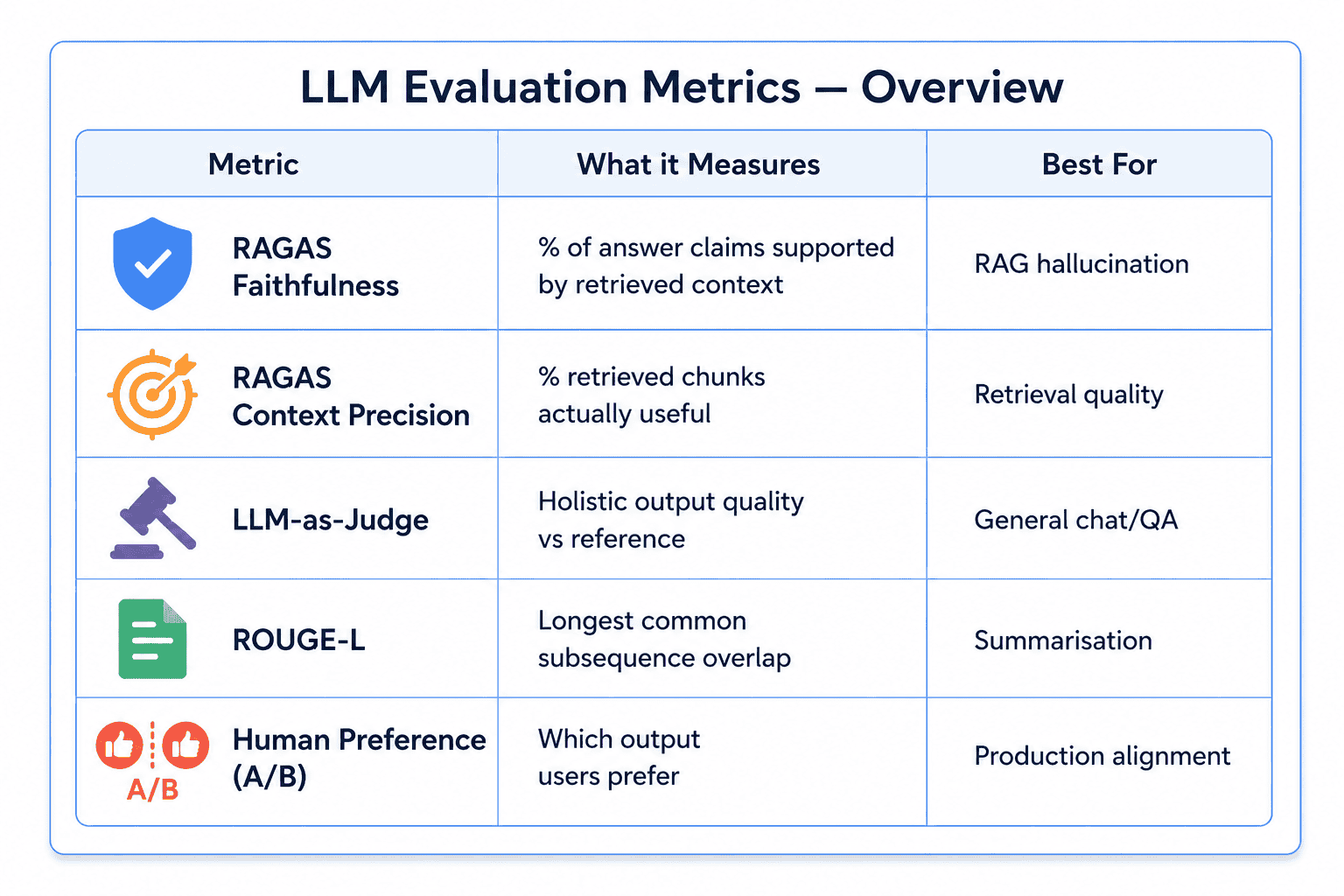
print(final.choices[0].message.content)Evaluating LLMs in production is far more complex than evaluating standard ML models because the outputs are open-ended and subjective.
Evaluation Framework:
- Automated Metrics: Using ROUGE, BLEU, or METEOR for summarization, and RAGAS for measuring RAG quality (Faithfulness, Relevance).
- LLM-as-a-Judge: Using a more powerful model (like GPT-4) to grade the responses of a smaller model based on predefined criteria.
- Human Evaluation: The gold standard. Blind A/B testing where humans rank the quality of different model outputs.
- Operational Metrics: Tracking token cost, latency (Time to First Token), and throughput.
# ── RAGAS — RAG evaluation framework ──────────────────────────────
from ragas import evaluate
from ragas.metrics import faithfulness, answer_relevancy, context_precision
from datasets import Dataset

# Your RAG pipeline outputs:
data = {
    "question":         ["What is our parental leave policy?"],
    "answer":           ["Employees get 16 weeks of paid parental leave."],
    "contexts":         [["Parental leave: full-time employees receive 16 weeks paid."]],
    "ground_truths":    [["16 weeks paid parental leave for all full-time staff."]],
}
results = evaluate(Dataset.from_dict(data),
                   metrics=[faithfulness, answer_relevancy, context_precision])
print(results)  # {"faithfulness": 1.0, "answer_relevancy": 0.95, ...}

# ── LLM-as-a-Judge  ────────────────────────────────────────────────
judge_prompt = """
Rate the answer on a scale 1–5 for: Correctness, Completeness, Conciseness.
Question:  {question}
Reference: {reference_answer}
Answer:    {model_answer}
Respond in JSON: {{"correctness": int, "completeness": int, "conciseness": int, "reasoning": str}}
"""
# Use GPT-4o or Claude as the judge — correlates well with human ratingsAs sequence lengths grow, the quadratic cost of standard attention becomes a bottleneck. Several innovations have emerged to optimize this.
Key Innovations:
- Flash Attention: An I/O-aware attention algorithm that uses tiling to compute attention without materializing the large N×N matrix, significantly speeding up training.
- Grouped-Query Attention (GQA): Shares single Key and Value heads across multiple Query heads, drastically reducing the memory footprint of the KV cache.
- Sliding Window Attention: Restricts each token to attending only to a local neighborhood, used in models like Mistral to handle longer contexts.
# Flash Attention via PyTorch SDPA (scaled dot product attention)
# Available in PyTorch ≥ 2.0 — auto-selects Flash Attention if available
import torch
import torch.nn.functional as F

q = torch.randn(2, 8, 512, 64, device='cuda', dtype=torch.bfloat16)  # (B, H, S, D)
k = torch.randn(2, 8, 512, 64, device='cuda', dtype=torch.bfloat16)
v = torch.randn(2, 8, 512, 64, device='cuda', dtype=torch.bfloat16)

# Automatically uses Flash Attention 2 kernel on supported hardware
with torch.backends.cuda.sdp_kernel(enable_flash=True, enable_math=False):
    out = F.scaled_dot_product_attention(q, k, v, is_causal=True)

# -- Grouped Query Attention (GQA) concept --
# Standard MHA: num_heads Q = num_heads K = num_heads V (e.g., 32/32/32)
# GQA:          num_heads Q > num_heads K = num_heads V (e.g., 32/8/8)
# KV cache size reduced by 4x in this example
# Hugging Face transformers uses GQA automatically for Llama 3:
from transformers import LlamaForCausalLM
model = LlamaForCausalLM.from_pretrained(
    "meta-llama/Llama-3-8B",
    attn_implementation="flash_attention_2",  # use FA2 kernel
    torch_dtype=torch.bfloat16
)Serving LLMs requires clever engineering to manage high VRAM requirements and compute-heavy inference.
Optimization Strategies:
- Quantization: Reducing weight precision (e.g., from 16-bit to 4-bit) to fit larger models on smaller GPUs with minimal accuracy loss (GPTQ, AWQ).
- Continuous Batching: Processing multiple requests simultaneously without waiting for the longest request in a batch to finish.
- PagedAttention: Storing the Key-Value (KV) cache in non-contiguous blocks (like OS virtual memory) to eliminate memory fragmentation (pioneered by vLLM).
# ── Quantisation with bitsandbytes (load in 4-bit) ─────────────────
from transformers import AutoModelForCausalLM, BitsAndBytesConfig
import torch

bnb_config = BitsAndBytesConfig(
    load_in_4bit=True,
    bnb_4bit_use_double_quant=True,
    bnb_4bit_quant_type="nf4",          # NormalFloat4 — optimal for LLMs
    bnb_4bit_compute_dtype=torch.bfloat16,
)
model = AutoModelForCausalLM.from_pretrained(
    "meta-llama/Llama-3-70B-Instruct",
    quantization_config=bnb_config,
    device_map="auto",                  # split across GPUs automatically
)

# ── vLLM — production inference server ──────────────────────────────
# pip install vllm
from vllm import LLM, SamplingParams

llm = LLM(
    model="meta-llama/Llama-3-8B-Instruct",
    tensor_parallel_size=2,             # 2 GPUs
    gpu_memory_utilization=0.90,
    quantization="awq",                 # AWQ 4-bit quantisation
)
params = SamplingParams(temperature=0.7, max_tokens=512)
outputs = llm.generate(prompts, params)   # continuous batching auto-managed

# ── Speculative Decoding ─────────────────────────────────────────────
# Small "draft" model (e.g., Llama-3-1B) generates K candidate tokens
# Large "target" model (e.g., Llama-3-70B) verifies all K in one forward pass
# Accepted tokens cost nothing extra; rejected tokens fall back to target sample
# Practical speedup: 2–3x on greedy/top-p decodingAI Alignment focuses on ensuring that an AI's goals and behaviors match human intentions and values.
Major Challenges:
- Reward Hacking: When a model finds a shortcut to get a high 'reward' without actually performing the desired task correctly.
- Scalable Oversight: Identifying how humans can supervise AI systems that become smarter than themselves in specialized domains.
- Distributional Shift: Ensuring a model that was aligned in a controlled environment stays aligned when deployed in the complex real world.
Hallucination is when an LLM generates factually incorrect information. In production engineering, we focus on both 'intrinsic' and 'extrinsic' hallucination.
Mitigation Strategies:
- Grounding: Forcing the model to reference specific retrieved documents (RAG).
- Chain of Verification (CoVe): Having the model double-check its own logic before finalizing the output.
- Self-Correction: Using a second LLM to 'audit' the first LLM's response for factual inconsistencies.
- Entropy/Uncertainty: Measuring the model's own confidence level; if it's low, the response is flagged for review.
# ── Self-Consistency Check ──────────────────────────────────────────
import openai, collections

client = openai.OpenAI()

def self_consistency_answer(question: str, n_samples: int = 10) -> dict:
    responses = []
    for _ in range(n_samples):
        r = client.chat.completions.create(
            model="gpt-4o",
            messages=[{"role": "user", "content": question}],
            temperature=0.7,  # need some randomness to show variance
        )
        responses.append(r.choices[0].message.content.strip())

    counts = collections.Counter(responses)
    most_common, count = counts.most_common(1)[0]
    confidence = count / n_samples
    return {
        "answer":     most_common,
        "confidence": confidence,     # 0.9 = high confidence, 0.3 = unreliable
        "all_samples": dict(counts),
    }

# ── Groundedness check with an LLM-as-judge ──────────────────────────
verification_prompt = """
Context: {retrieved_context}
Claim: {model_answer}

Is every factual claim in 'Claim' supported by 'Context'?
Reply JSON: {{"supported": true/false, "unsupported_claims": [list]}}
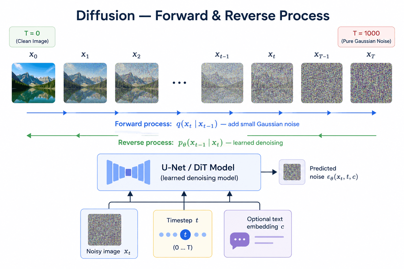
"""Diffusion models are the backbone of modern image generation (Stable Diffusion, Midjourney). They learn to generate data by reversing a noise-addition process.
Phases of Training:
- Forward Diffusion: Gradually adding Gaussian noise to a clean image until it becomes unrecognizable.
- Reverse Diffusion: Training a neural network (typically a U-Net) to 'denoise' the image step by step.
- Conditioning: Injecting text embeddings (via cross-attention) so the model learns to associate specific visuals with specific words.
import torch
import torch.nn.functional as F

# ── Forward Process: add noise at timestep t ───────────────────────
def q_sample(x0, t, noise, alphas_cumprod):
    """
    x0: clean image tensor
    t:  timestep (integer 0..T)
    Returns: noisy image x_t
    """
    alpha_t    = alphas_cumprod[t].view(-1, 1, 1, 1)
    sqrt_alpha = alpha_t.sqrt()
    sqrt_one_minus_alpha = (1 - alpha_t).sqrt()
    return sqrt_alpha * x0 + sqrt_one_minus_alpha * noise

# ── Training Loop (simplified DDPM loss) ──────────────────────────
def train_step(model, x0, alphas_cumprod, T=1000):
    t     = torch.randint(0, T, (x0.shape[0],))       # random timestep per batch
    noise = torch.randn_like(x0)                       # target noise
    x_t   = q_sample(x0, t, noise, alphas_cumprod)    # noisy image

    # Model predicts the noise added at step t
    noise_pred = model(x_t, t)

    loss = F.mse_loss(noise_pred, noise)               # L2 loss on noise
    return loss

# ── Inference: iterative denoising (DDPM sampler) ─────────────────
@torch.no_grad()
def sample(model, T, alphas, betas, shape):
    x = torch.randn(shape)                   # start from random noise
    for t in reversed(range(T)):
        noise_pred = model(x, torch.tensor([t]))
        # Compute denoised estimate and add controlled noise for stochasticity
        x = ddpm_reverse_step(x, t, noise_pred, alphas, betas)
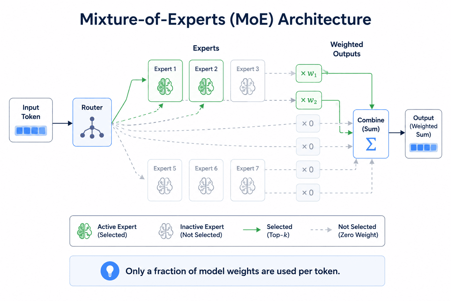
return x # final clean imageMixture-of-Experts (MoE) is an architecture (like Mixtral or GPT-4) that allows for very large models to remain efficient during inference.
Core Concepts:
- Sparse Activation: Instead of using every neuron for every token, the model only activates a small 'expert' subset (typically 2 out of 8).
- Router: A gating network that decides which experts are best suited to process a given token.
- Performance: You get the knowledge capacity of a massive model (e.g., 1T params) with the inference speed and cost of a much smaller one (e.g., 10B params).
import torch
import torch.nn as nn
import torch.nn.functional as F

class MoELayer(nn.Module):
    def __init__(self, d_model, d_ff, n_experts=8, top_k=2):
        super().__init__()
        self.router   = nn.Linear(d_model, n_experts)     # gating network
        self.experts  = nn.ModuleList([
            nn.Sequential(nn.Linear(d_model, d_ff), nn.SiLU(), nn.Linear(d_ff, d_model))
            for _ in range(n_experts)
        ])
        self.top_k = top_k

    def forward(self, x):
        # x: (batch, seq_len, d_model)
        B, S, D = x.shape
        x_flat  = x.view(-1, D)                                 # (B*S, D)

        # Route: get top-K expert probabilities per token
        logits  = self.router(x_flat)                           # (N, n_experts)
        probs, indices = torch.topk(F.softmax(logits, dim=-1), self.top_k, dim=-1)

        # Dispatch tokens to their selected experts
        output = torch.zeros_like(x_flat)
        for k in range(self.top_k):
            expert_idx = indices[:, k]                          # (N,)
            weight     = probs[:, k].unsqueeze(-1)              # (N, 1)
            for e_id in range(len(self.experts)):
                mask    = (expert_idx == e_id)
                if mask.any():
                    output[mask] += weight[mask] * self.experts[e_id](x_flat[mask])
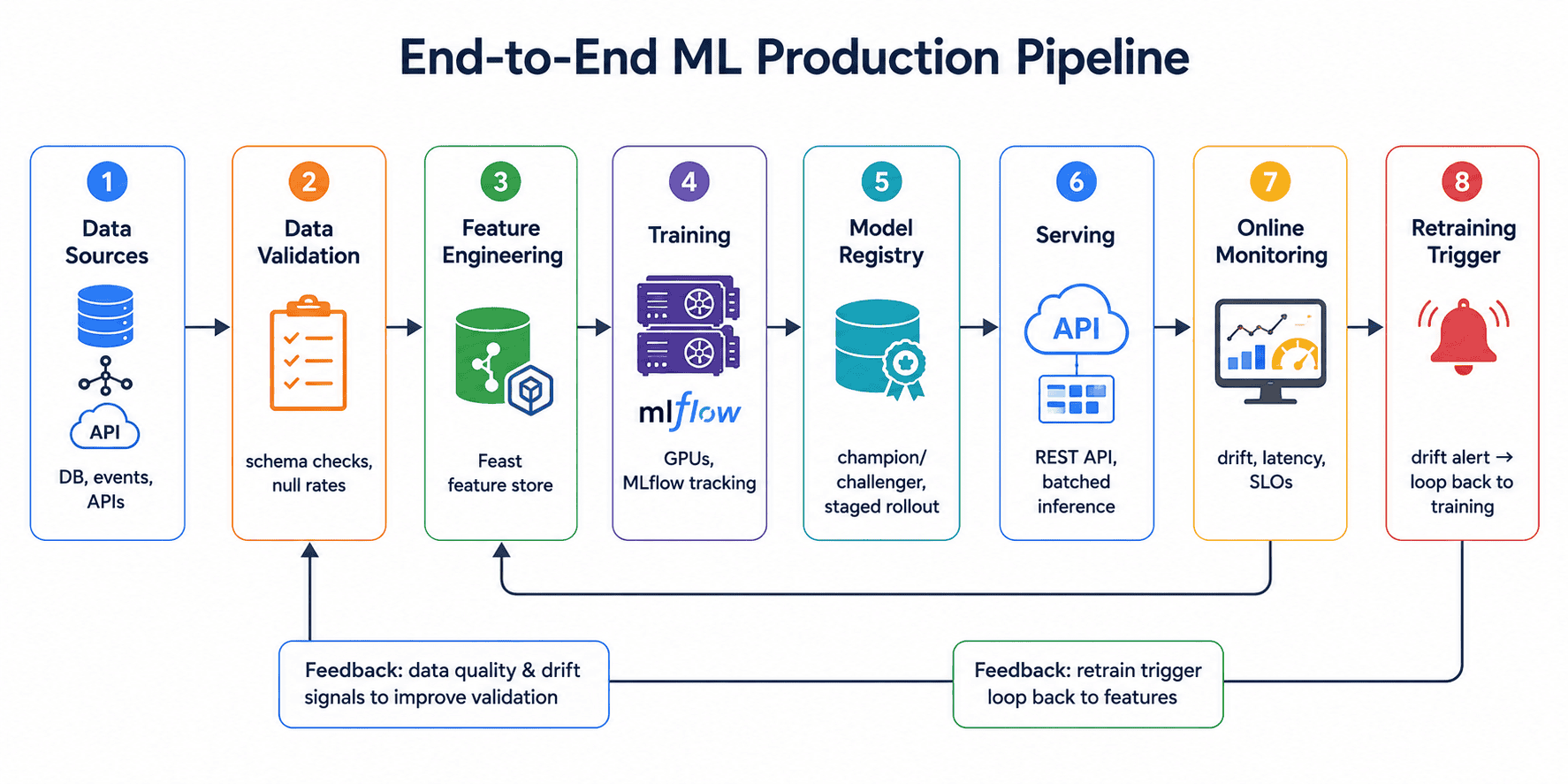
return output.view(B, S, D)A production ML pipeline includes: data ingestion + validation (Pandera/Great Expectations), feature engineering (Feast), model training + experiment tracking (MLflow/W&B), model registry + versioning, deployment (REST API via FastAPI/TorchServe, or streaming via Kafka), online monitoring (data drift detection — PSI, KS test; prediction drift; latency/error SLOs), and automated retraining triggers. Infrastructure: Kubernetes + Helm for orchestration, Airflow or Prefect for scheduling.
# ── Data Drift Detection (Population Stability Index) ─────────────
import numpy as np

def psi(expected: np.ndarray, actual: np.ndarray, buckets: int = 10) -> float:
    """
    PSI < 0.1:  No significant shift
    PSI 0.1–0.2: Moderate shift; investigate
    PSI > 0.2:  Major shift; consider retraining
    """
    breakpoints = np.percentile(expected, np.linspace(0, 100, buckets + 1))
    expected_pct = np.histogram(expected, bins=breakpoints)[0] / len(expected) + 1e-10
    actual_pct   = np.histogram(actual,   bins=breakpoints)[0] / len(actual)   + 1e-10
    return float(np.sum((actual_pct - expected_pct) * np.log(actual_pct / expected_pct)))

# ── MLflow Experiment Tracking ────────────────────────────────────
import mlflow

with mlflow.start_run(run_name="llama-ft-v3"):
    mlflow.log_params({"lr": 1e-4, "batch_size": 16, "epochs": 3, "lora_r": 16})
    for epoch, metrics in enumerate(training_loop()):
        mlflow.log_metrics(metrics, step=epoch)
    mlflow.pytorch.log_model(model, "model", registered_model_name="llama-ft")

# ── Promote champion in model registry ────────────────────────────
client = mlflow.tracking.MlflowClient()
client.transition_model_version_stage(
    name="llama-ft", version=3, stage="Production"
)Responsible AI covers: Bias — systematic unfairness in model predictions across demographic groups, arising from biased training data, label bias, or feedback loops. Fairness metrics: Demographic Parity, Equalised Odds, Individual Fairness. Mitigation: diverse training data, re-sampling, adversarial debiasing, post-processing calibration. Privacy: differential privacy, federated learning. Transparency: model cards, explainability (SHAP, LIME, attention maps). Governance: AI audit trails, human-in-the-loop for high-stakes decisions.
# ── Fairness Evaluation with Fairlearn ────────────────────────────
from fairlearn.metrics import MetricFrame, demographic_parity_difference
from sklearn.metrics import accuracy_score

metric_frame = MetricFrame(
    metrics={"accuracy": accuracy_score},
    y_true=y_test,
    y_pred=y_pred,
    sensitive_features=X_test["gender"],  # protected attribute
)
print(metric_frame.by_group)   # accuracy broken down by group
print(demographic_parity_difference(y_test, y_pred,
                                    sensitive_features=X_test["gender"]))

# ── SHAP — model explainability ─────────────────────────────────────
import shap

explainer  = shap.Explainer(model, X_train)
shap_values = explainer(X_test)

# Feature importance plot — which features drive predictions?
shap.plots.bar(shap_values)

# Waterfall plot — why did THIS specific prediction happen?
shap.plots.waterfall(shap_values[0])

# ── Differential Privacy (during training) ────────────────────────
from opacus import PrivacyEngine

privacy_engine = PrivacyEngine()
model_dp, optimizer_dp, loader_dp = privacy_engine.make_private(
    module=model,
    optimizer=optimizer,
    data_loader=train_loader,
    noise_multiplier=1.2,  # controls privacy-utility tradeoff
    max_grad_norm=1.0,     # clips per-sample gradients
)
# After training:
epsilon = privacy_engine.get_epsilon(delta=1e-5)
print(f"(ε={epsilon:.1f}, δ=1e-5)-DP guarantee achieved")The most valued skill in AI engineering is knowing when not to use a neural network. If an interviewer gives you a problem, ask: can we solve this with a rule-based system, a simple logistic regression, or an off-the-shelf API first? Showing this judgment signals production maturity.
No technique is universally correct. When asked about RAG vs Fine-tuning, or prompting vs RLHF, structure your answer as: “It depends on X, Y, Z. If [condition], I'd choose [approach] because [reason].” Interviewers test whether you think in systems, not textbooks.
Every system design answer should end with: “And here's how I'd evaluate and monitor this in production.” Explain your metrics (online + offline), your retraining triggers, and your deployment strategy. Candidates who skip evaluation are seen as academically focused, not production-ready.
Be fluent with the tools the industry actually uses: vLLM, LangChain/LangGraph, HuggingFace Transformers, PEFT/LoRA, MLflow/W&B, FAISS/Qdrant. Being able to name the library and explain why you'd choose it over alternatives demonstrates that your knowledge is practical, not theoretical.
The AI engineering landscape has evolved rapidly — the best engineers in 2026 combine strong ML fundamentals with hands-on experience building LLM systems that work reliably at production scale. Mastering these 25 questions will give you the vocabulary, depth, and practical confidence to excel in any AI engineer interview.
Build hands-on experience with the Hugging Face ecosystem, LangChain, and an open-source model like Llama 3. Set up a small RAG project or fine-tune a model on a custom dataset — a demo you can walk through is worth 10 text-book answers. Good luck!
Explore more resources →Md Rashid
Software engineer and career coach with 6+ years in the tech industry. Writes about interview prep, developer careers, and tech job markets.
Top 25 Machine Learning Interview Questions and Answers (2026 Edition)
Ace your next ML interview with this comprehensive guide covering decision trees, gradient boosting, SVMs, clustering, regularisation, causal inference, conformal prediction, and production ML system design.

Highest Paying Tech Jobs in 2026
Discover the 10 highest-paying tech roles available right now, with real salary data, clear breakdowns of what each job involves, who each role suits best, and actionable advice on how to break in — even from zero experience.
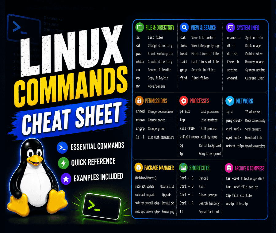
The Complete Linux Commands Cheat Sheet 2026
Every essential Linux command defined with clean, practical examples. Covers file navigation, system monitoring, user permissions, networking, package management, and shell scripting.
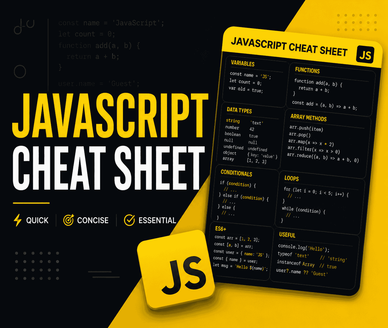
The Complete JavaScript Cheat Sheet 2026
Every essential JavaScript syntax, method, and pattern you need — from variables, arrays, and objects to async/await, closures, ES2026 features, and DOM manipulation. Clean, copy-paste-ready examples.