
Whether you’re interviewing for a data scientist, ML engineer, or applied scientist role, this guide covers the concepts that appear most often across technical screens at top tech companies and AI-native startups — from foundational theory to advanced production system design.
A machine learning interview evaluates three overlapping competencies:
The 25 questions below are organised by difficulty and span all three competencies — from the bias-variance tradeoff through Gaussian processes and real-time fraud detection system design.
Parametric models assume a fixed functional form with a set number of parameters that do not change regardless of the amount of data. Once the parameters are learned, you can discard the training data.
Key characteristics of Parametric models:
- Fixed functional form (e.g., y = mx + c).
- Constant number of parameters.
- Faster at inference as they only require parameters.
- Examples: Linear Regression, Logistic Regression, Naive Bayes.
Non-parametric models make no fixed assumptions about the form of the mapping function. They are flexible and the number of parameters grows with the size of the data.
Key characteristics of Non-parametric models:
- No fixed assumptions about the underlying distribution.
- Flexibility to fit complex patterns.
- Require more training data and are usually slower at inference.
- Examples: k-Nearest Neighbors (k-NN), Decision Trees, SVM with RBF kernel.
| Property | Parametric | Non-Parametric |
|---|---|---|
| Model Form | Fixed assumptions | Flexible |
| Parameters | Fixed count | Grows with data |
| Memory at inference | Params only | Needs training data |
| Training data needed | Less | More |
| Examples | Linear Regression, Logistic Regression, Naive Bayes | k-NN, Decision Tree, Kernel SVM, Gaussian Process |
Comparison of model properties between parametric and non-parametric approaches.
Generative models learn the joint probability distribution P(x, y) and model how the data was generated. They can be used to generate new samples by calculating P(x|y).
Characteristics of Generative models:
- Model the distribution of individual classes.
- Useful for synthesizing data and handling missing values.
- Examples: Naive Bayes, Gaussian Mixture Models (GMM), GANs, VAEs.
Discriminative models learn the decision boundary directly by modeling P(y|x). They focus on separating different classes rather than understanding how they are built.
Characteristics of Discriminative models:
- Focus on the boundary between classes.
- Usually achieve higher classification accuracy.
- Examples: Logistic Regression, Support Vector Machines (SVM), Neural Networks.
| Property | Generative | Discriminative |
|---|---|---|
| What it models | Joint distribution P(x, y) | Conditional P(y | x) |
| Goal | Understand how data is generated | Maximise class separation |
| New sample generation | Yes — can synthesise new data | No |
| Missing feature handling | Graceful (marginalise out) | Difficult |
| Typical accuracy | Moderate | Higher |
| Examples | Naive Bayes, GMM, GAN, VAE | Logistic Regression, SVM, Neural Network |
Side-by-side comparison of generative and discriminative model properties.
A decision tree splits nodes by finding the attribute that results in the cleanest separation of classes. It uses various metrics to decide where to split:
Key Concepts:
- Entropy: A measure of disorder or impurity in a set of data. High entropy means high impurity.
- Information Gain: The reduction in entropy achieved by partitioning the data according to a specific feature.
- Gini Impurity: Used by CART (Classification and Regression Trees), it measures the frequency at which a randomly chosen element from the set would be incorrectly labeled if it was randomly labeled according to the distribution of labels in the subset.
import numpy as np

def entropy(y):
    classes, counts = np.unique(y, return_counts=True)
    p = counts / len(y)
    return -np.sum(p * np.log2(p + 1e-9))

def information_gain(y_parent, y_left, y_right):
    n = len(y_parent)
    weighted_child_entropy = (
        len(y_left)  / n * entropy(y_left) +
        len(y_right) / n * entropy(y_right)
    )
    return entropy(y_parent) - weighted_child_entropy

# Gini impurity: 1 - sum(p_i^2)
def gini(y):
    _, counts = np.unique(y, return_counts=True)
    p = counts / len(y)
    return 1 - np.sum(p ** 2)

# sklearn decision tree (uses Gini by default)
from sklearn.tree import DecisionTreeClassifier
dt = DecisionTreeClassifier(criterion='gini', max_depth=5, min_samples_leaf=10)
dt.fit(X_train, y_train)Regularisation is a technique used to prevent overfitting by adding a penalty term to the cost function. This discourages the model from learning overly complex patterns.
L1 Regularisation (Lasso):
- Adds the 'absolute value of magnitude' of coefficients as a penalty term.
- Can lead to zero-weight coefficients, effectively performing feature selection.
- Better for models where you suspect only a few features are important.
L2 Regularisation (Ridge):
- Adds the 'squared magnitude' of coefficients as a penalty term.
- Shrinks coefficients towards zero but rarely makes them exactly zero.
- Better for models where many features contribute small amounts to the prediction.
| Property | L1 (Lasso) | L2 (Ridge) |
|---|---|---|
| Penalty term | Σ|wᵢ| (absolute values) | Σwᵢ² (squared values) |
| Effect on weights | Shrinks to exactly zero | Shrinks toward zero, never exactly |
| Feature selection | Yes — sparse solution | No — keeps all features |
| Best when | Few features matter | Many features contribute small amounts |
| sklearn class | Lasso / LassoCV | Ridge / RidgeCV |
Key differences between L1 and L2 regularisation techniques.
# Loss = MSE + λ * penalty
# L1 (Lasso):    penalty = Σ|wᵢ|       → sparse weights (feature selection)
# L2 (Ridge):    penalty = Σwᵢ²        → small but non-zero weights
# ElasticNet:    penalty = α*Σ|wᵢ| + (1-α)*Σwᵢ²

from sklearn.linear_model import Lasso, Ridge, ElasticNet
from sklearn.pipeline import Pipeline
from sklearn.preprocessing import StandardScaler

# Always scale features before regularisation — penalty is scale-sensitive!
lasso = Pipeline([
    ("scaler", StandardScaler()),
    ("model",  Lasso(alpha=0.1))        # alpha = λ (regularisation strength)
])
ridge = Pipeline([
    ("scaler", StandardScaler()),
    ("model",  Ridge(alpha=1.0))
])

# Selecting alpha via cross-validation
from sklearn.linear_model import LassoCV, RidgeCV
lasso_cv = LassoCV(cv=5).fit(X_train, y_train)
print(f"Best alpha: {lasso_cv.alpha_:.4f}")
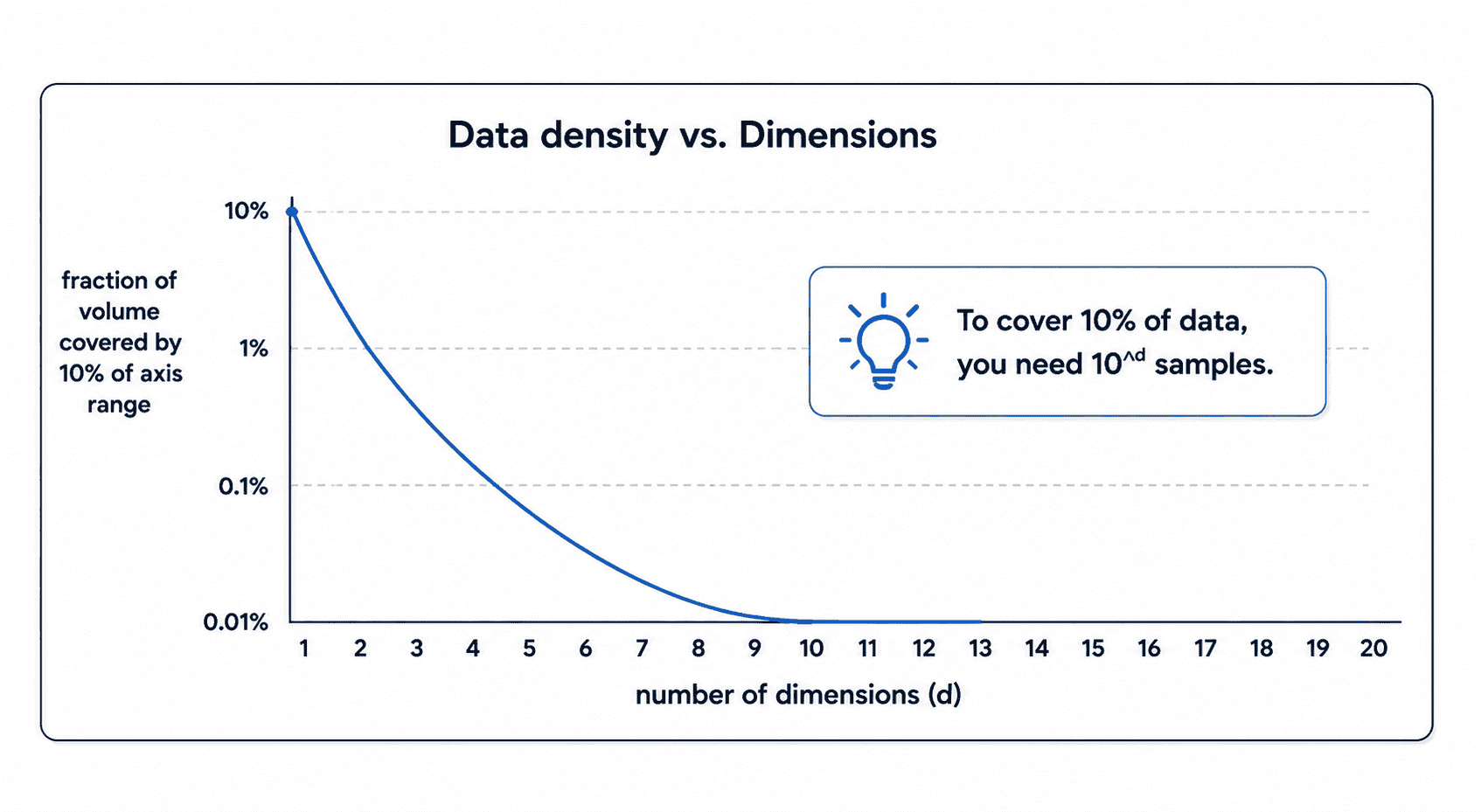
print(f"Non-zero features: {(lasso_cv.coef_ != 0).sum()}")The curse of dimensionality refers to the various phenomena that arise when analyzing data in high-dimensional spaces that do not occur in low-dimensional settings.
Major Impacts:
- Data Sparsity: As dimensions increase, the volume of the space increases so fast that available data becomes sparse.
- Distance Metrics: In high dimensions, the distance between any two points becomes almost the same, making clustering or nearest-neighbor algorithms ineffective.
- Overfitting: With more features, it's easier for a model to find a hyperplane that separates the data perfectly but doesn't generalize.
Bagging and Boosting are both ensemble techniques used to combine multiple weak learners to create a strong learner.
Bagging (Bootstrap Aggregating):
- Trees are built in parallel.
- Each tree is trained on a random subset of data (with replacement).
- Aim: Reduce variance (overfitting).
- Example: Random Forest.
Boosting:
- Trees are built sequentially.
- Each new tree attempts to correct the errors of the previous ones.
- Aim: Reduce bias (underfitting).
- Example: AdaBoost, Gradient Boosting, XGBoost.
| Property | Bagging | Boosting |
|---|---|---|
| Tree building order | Parallel | Sequential |
| Data sampling | Bootstrap samples (with replacement) | Full data; upweights misclassified points |
| Primary goal | Reduce variance (overfitting) | Reduce bias (underfitting) |
| Model independence | Trees are independent | Each tree depends on the previous |
| Sensitive to outliers | Low | Higher (outliers gain more weight) |
| Example algorithms | Random Forest | AdaBoost, XGBoost, LightGBM |
Side-by-side comparison of bagging and boosting ensemble strategies.
k-NN is a simple, instance-based learning algorithm. It classifies a point based on the majority class of its 'k' nearest neighbors in the feature space.
Steps:
1. Choose the number 'k' and a distance metric (e.g., Euclidean).
2. Find the k nearest neighbors of the new point.
3. Assign the class that is most common among those neighbors.
Limitations:
- Computationally expensive at inference time (O(n)).
- Sensitive to irrelevant features and data scaling.
- Requires significant memory to store the entire training dataset.
from sklearn.neighbors import KNeighborsClassifier
from sklearn.preprocessing import StandardScaler
from sklearn.model_selection import cross_val_score
import numpy as np

# k-NN is scale-sensitive — always normalise!
scaler = StandardScaler()
X_train_s = scaler.fit_transform(X_train)
X_test_s  = scaler.transform(X_test)

# Choose k via cross-validation
k_scores = [
    cross_val_score(KNeighborsClassifier(n_neighbors=k), X_train_s, y_train,
                    cv=5, scoring='accuracy').mean()
    for k in range(1, 31)
]
best_k = np.argmax(k_scores) + 1          # 1-indexed
print(f"Best k: {best_k}, CV acc: {k_scores[best_k-1]:.3f}")

knn = KNeighborsClassifier(n_neighbors=best_k, metric='euclidean')
knn.fit(X_train_s, y_train)

# Speed up with KD-Tree or Ball-Tree for low dimensions (d < 20)
knn_fast = KNeighborsClassifier(n_neighbors=best_k, algorithm='kd_tree')PCA is a dimensionality reduction technique that transforms a large set of variables into a smaller one that still contains most of the information in the original set.
How it works:
1. Standardize the data.
2. Compute the covariance matrix to identify correlations.
3. Calculate eigenvectors and eigenvalues to find principal components (directions of maximum variance).
4. Sort eigenvectors by eigenvalue and choose the top 'k' components.
5. Project original data into the new subspace.
from sklearn.decomposition import PCA
from sklearn.preprocessing import StandardScaler
import matplotlib.pyplot as plt
import numpy as np

# Always scale before PCA — variance is scale-dependent
scaler = StandardScaler()
X_scaled = scaler.fit_transform(X)

# Fit PCA and inspect explained variance
pca = PCA()
pca.fit(X_scaled)

# Choose n_components: cumulative explained variance >= 95%
cumvar = np.cumsum(pca.explained_variance_ratio_)
n_components = np.argmax(cumvar >= 0.95) + 1
print(f"Components for 95% variance: {n_components}")

# Plot scree plot
plt.plot(cumvar)
plt.axhline(0.95, color='r', linestyle='--', label='95% variance')
plt.xlabel('Number of Components'); plt.ylabel('Cumulative Explained Variance')
plt.legend(); plt.show()

# Apply reduction
pca_final = PCA(n_components=n_components)
X_reduced = pca_final.fit_transform(X_scaled) # shape: (n_samples, n_components)SVM separates data points of different classes using a hyperplane that has the maximum margin. The goal is to maximize the distance between the hyperplane and the nearest data points of each class (the support vectors).
Key Concepts:
- Maximum Margin: SVM finds the 'widest street' that separates classes.
- Support Vectors: Data points that lie closest to the hyperplane; if moved, the boundary would change.
- Kernel Trick: For data that isn't linearly separable, the kernel trick maps the input features into a higher-dimensional space where a linear separator can be found.
Common Kernels:
- Linear: Simple dot product.
- Polynomial: For curved boundaries.
- RBF (Gaussian): Powerful for complex, non-linear boundaries.
from sklearn.svm import SVC
from sklearn.preprocessing import StandardScaler
from sklearn.model_selection import GridSearchCV
from sklearn.pipeline import Pipeline

# SVM is scale-sensitive — always normalise
pipe = Pipeline([
    ("scaler", StandardScaler()),
    ("svm",    SVC(probability=True))
])

# Grid search over C (regularisation) and gamma (RBF width)
param_grid = {
    "svm__C":      [0.1, 1, 10, 100],     # C: margin width vs misclassification
    "svm__gamma":  ["scale", 0.001, 0.01], # gamma: how far influence of each point reaches
    "svm__kernel": ["rbf", "linear"],
}
search = GridSearchCV(pipe, param_grid, cv=5, scoring="f1_macro", n_jobs=-1)
search.fit(X_train, y_train)
print(f"Best params: {search.best_params_}")
print(f"Best CV F1:  {search.best_score_:.3f}")

# Insight: large C = narrow hard margin (risk overfit)
#          small C = wide soft margin (risk underfit)
# large gamma = each point has narrow influence (overfit)
# small gamma = each point has wide influence (underfit)Gradient Boosting is an ensemble method that builds models sequentially. Each new model (usually a decision tree) tries to predict and correct the errors (residuals) of the previous models.
XGBoost (Extreme Gradient Boosting) Key Improvements:
- Regularization: Built-in L1 and L2 regularization to prevent overfitting.
- Handling Missing Data: Automatically learns the best way to handle missing values.
- Tree Pruning: Uses a 'depth-first' approach and prunes trees backward.
- Hardware Optimization: Utilizes parallel processing and cache-aware access for extreme speed.
import xgboost as xgb
from sklearn.model_selection import cross_val_score
import optuna

# Basic XGBoost usage
model = xgb.XGBClassifier(
    n_estimators=500,
    learning_rate=0.05,       # shrinkage — lower = better generalisation, needs more trees
    max_depth=6,              # tree depth — controls complexity
    subsample=0.8,            # row subsampling per tree
    colsample_bytree=0.8,     # feature subsampling per tree
    reg_alpha=0.1,            # L1 regularisation on leaf weights
    reg_lambda=1.0,           # L2 regularisation on leaf weights
    eval_metric="logloss",
    early_stopping_rounds=50,
    random_state=42,
    device="cuda",            # GPU training
)
model.fit(X_train, y_train,
          eval_set=[(X_val, y_val)],
          verbose=False)

# Hyperparameter tuning with Optuna (Bayesian optimisation)
def objective(trial):
    params = {
        "max_depth":        trial.suggest_int("max_depth", 3, 10),
        "learning_rate":    trial.suggest_float("lr", 0.01, 0.3, log=True),
        "subsample":        trial.suggest_float("subsample", 0.5, 1.0),
        "colsample_bytree": trial.suggest_float("colsample_bytree", 0.5, 1.0),
    }
    m = xgb.XGBClassifier(**params, n_estimators=300, random_state=42)
    return cross_val_score(m, X_train, y_train, cv=5, scoring="roc_auc").mean()

study = optuna.create_study(direction="maximize")
study.optimize(objective, n_trials=50)The EM algorithm is an iterative strategy for finding maximum likelihood estimates of parameters in models with latent (hidden) variables.
The Two Steps:
1. Expectation (E) step: Estimate the missing or latent variables given the current parameters.
2. Maximisation (M) step: Update the parameters of the model to maximize the likelihood of the data, assuming the latent variables from the E-step are correct.
Common Applications:
- Gaussian Mixture Models (GMM) for clustering.
- Hidden Markov Models (HMM).
- Missing data imputation.
from sklearn.mixture import GaussianMixture
import numpy as np

# EM is the algorithm under the hood of GMM
# E-step: assign soft cluster probabilities to each point
# M-step: update cluster means, covariances, and weights

gmm = GaussianMixture(
    n_components=3,          # number of Gaussian clusters
    covariance_type='full',  # each cluster has its own covariance matrix
    max_iter=200,
    n_init=10,               # run 10 random inits; keep best
    random_state=42
)
gmm.fit(X)

# Soft cluster assignments (posterior probabilities)
probs   = gmm.predict_proba(X)    # shape (n, 3)
labels  = gmm.predict(X)          # hard assignments (argmax)
score   = gmm.score(X)            # log-likelihood per sample

# Choose number of components with BIC (penalises complexity)
bics = [GaussianMixture(n_components=k, n_init=5).fit(X).bic(X)
        for k in range(1, 11)]
best_k = np.argmin(bics) + 1
print(f"Best k by BIC: {best_k}")Feature engineering starts with raw data and creates meaningful features that help algorithms learn better. It often provides the biggest boost in model performance.
Key Techniques:
- Categorical Encoding: One-hot encoding, Label encoding, Target encoding.
- Interaction Features: Creating features by combining two or more existing ones (e.g., price x quantity).
- Feature Scaling: Normalization or Standardization (critical for k-NN, SVM, Neural Nets).
- Dimensionality Reduction: PCA or LDA to reduce noise and redundancy.
- Domain-Specific Transformation: Extracting 'hour' from a timestamp or 'domain' from an email.
import pandas as pd
import numpy as np
from sklearn.preprocessing import TargetEncoder, PolynomialFeatures

df = pd.read_csv("data.csv")

# ── Categorical Encoding ────────────────────────────────────────────
# One-hot (low cardinality)
df = pd.get_dummies(df, columns=["color"], drop_first=True)

# Target encoding (high cardinality — e.g., zip code, user_id)
enc = TargetEncoder(smooth="auto")
df["city_encoded"] = enc.fit_transform(df[["city"]], df["target"])

# ── Numeric Transforms ──────────────────────────────────────────────
df["log_price"]   = np.log1p(df["price"])       # handles 0s safely
df["sqrt_area"]   = np.sqrt(df["area"])
df["price_per_m2"] = df["price"] / df["area"]   # ratio feature

# ── Date/Time Decomposition ─────────────────────────────────────────
df["timestamp"] = pd.to_datetime(df["timestamp"])
df["hour"]      = df["timestamp"].dt.hour
df["dayofweek"] = df["timestamp"].dt.dayofweek
df["is_weekend"]= (df["dayofweek"] >= 5).astype(int)

# ── Group Aggregation Features ──────────────────────────────────────
agg = df.groupby("customer_id")["amount"].agg(["mean","std","count"])
agg.columns = ["cust_avg_amount","cust_std_amount","cust_txn_count"]
df = df.merge(agg, on="customer_id", how="left")

# ── Polynomial Interactions ─────────────────────────────────────────
poly = PolynomialFeatures(degree=2, interaction_only=True)
X_poly = poly.fit_transform(X_numeric)Imbalanced datasets occur when one class has significantly more samples than another, causing the model to biassed toward the majority class.
Techniques to mitigate this:
- Resampling: Oversampling the minority class (e.g., SMOTE) or undersampling the majority class.
- Algorithm-level tuning: Using 'balanced' class weights in algorithms like Random Forest or SVM.
- Evaluation Metrics: Using Precision-Recall or F1-score instead of Accuracy.
- Threshold Moving: Adjusting the decision threshold to favor the minority class.
from imblearn.over_sampling import SMOTE
from imblearn.pipeline import Pipeline as ImbPipeline
from sklearn.ensemble import RandomForestClassifier
from sklearn.metrics import classification_report

# ── Method 1: SMOTE oversampling ────────────────────────────────────
smote = SMOTE(sampling_strategy=0.5, random_state=42)
X_res, y_res = smote.fit_resample(X_train, y_train)
print(f"Before: {y_train.value_counts().to_dict()}")
print(f"After:  {pd.Series(y_res).value_counts().to_dict()}")

# ── Method 2: class_weight='balanced' (easiest, usually effective) ──
rf = RandomForestClassifier(class_weight='balanced', n_estimators=200)
rf.fit(X_train, y_train)

# ── Method 3: Threshold tuning ──────────────────────────────────────
from sklearn.metrics import precision_recall_curve
probs = rf.predict_proba(X_test)[:, 1]

precisions, recalls, thresholds = precision_recall_curve(y_test, probs)
# Find threshold that maximises F1
f1_scores = 2 * (precisions * recalls) / (precisions + recalls + 1e-9)
best_thresh = thresholds[f1_scores[:-1].argmax()]
print(f"Optimal threshold: {best_thresh:.3f}")
y_pred_tuned = (probs >= best_thresh).astype(int)
print(classification_report(y_test, y_pred_tuned))The choice depends on whether your model needs to adapt to new data in real-time or if it can be updated on a schedule.
Batch Learning:
- The model is trained on the entire dataset at once.
- Retraining is expensive and requires the whole dataset.
- Suitable for static data where patterns don't change quickly.
Online (Incremental) Learning:
- The model is updated continuously as new data arrives.
- Examples include Stochastic Gradient Descent (SGD) or online Bayesian models.
- Ideal for streaming data or scenarios with limited memory (cannot load all data at once).
| Property | Batch Learning | Online Learning |
|---|---|---|
| Training trigger | Scheduled (e.g., nightly) | Continuous — each new sample |
| Data requirement | Full dataset in memory | One sample (or mini-batch) at a time |
| Retraining cost | High — full retrain needed | Low — incremental update |
| Adapts to drift | Only after retraining | Immediately |
| Best for | Static data, stable distributions | Streaming data, concept drift |
| Examples | Scikit-learn RandomForest, XGBoost | SGDClassifier, River library |
Comparison of batch and online (incremental) learning paradigms.
from sklearn.linear_model import SGDClassifier
from sklearn.preprocessing import StandardScaler
import numpy as np

# SGDClassifier supports partial_fit — true online learning
scaler = StandardScaler()
clf    = SGDClassifier(loss='log_loss', learning_rate='adaptive',
                       eta0=0.01, random_state=42)

# Simulate a data stream arriving in chunks
def stream_data(X, y, chunk_size=256):
    for i in range(0, len(X), chunk_size):
        yield X[i:i+chunk_size], y[i:i+chunk_size]

classes = np.unique(y_train)    # must pass all classes on first call
first_chunk = True
for X_chunk, y_chunk in stream_data(X_train, y_train):
    X_chunk_s = scaler.partial_fit(X_chunk).transform(X_chunk)
    if first_chunk:
        clf.partial_fit(X_chunk_s, y_chunk, classes=classes)
        first_chunk = False
    else:
        clf.partial_fit(X_chunk_s, y_chunk)

# River — dedicated online ML library
from river import linear_model, preprocessing, metrics
model = preprocessing.StandardScaler() | linear_model.LogisticRegression()
metric = metrics.ROCAUC()
for x, y in river_dataset:
    y_pred = model.predict_proba_one(x)
    metric.update(y, y_pred)
model.learn_one(x, y)Linear regression (OLS) relies on several key assumptions to ensure the coefficient estimates are reliable and unbiased.
Core Assumptions:
1. Linearity: The relationship between independent and dependent variables is linear.
2. Independence: Observations are independent of each other.
3. Homoscedasticity: The variance of residual errors is constant across all levels of the independent variables.
4. Normality: The residual errors are normally distributed (important for confidence intervals).
5. No Multicollinearity: Independent variables should not be highly correlated with each other.
import numpy as np
import statsmodels.api as sm
import matplotlib.pyplot as plt
from scipy import stats

X_sm = sm.add_constant(X_train)   # adds intercept column
model = sm.OLS(y_train, X_sm).fit()
print(model.summary())             # coefficients, p-values, R², AIC

residuals = model.resid
fitted    = model.fittedvalues

# 1. Residuals vs Fitted  — checks linearity & homoscedasticity
plt.scatter(fitted, residuals); plt.axhline(0, color='r')
plt.xlabel("Fitted"); plt.ylabel("Residuals"); plt.title("Residuals vs Fitted")

# 2. Q-Q plot — checks normality of residuals
sm.qqplot(residuals, line='s'); plt.title("Q-Q Plot")

# 3. Breusch-Pagan test — formal homoscedasticity test
from statsmodels.stats.diagnostic import het_breuschpagan
bp_test = het_breuschpagan(residuals, X_sm)
print(f"BP p-value: {bp_test[1]:.4f}")   # p < 0.05 → heteroscedasticity

# 4. VIF — detects multicollinearity
from statsmodels.stats.outliers_influence import variance_inflation_factor
vif = [variance_inflation_factor(X_sm.values, i) for i in range(X_sm.shape[1])]
print("VIF:", vif) # VIF > 10 → severe multicollinearityk-Means is an unsupervised learning algorithm that partitions 'n' observations into 'k' clusters by minimizing the distance between points and their cluster centroids.
How it works:
1. Randomly initialize 'k' centroids.
2. Assign each data point to the nearest centroid (typically using Euclidean distance).
3. Recalculate centroids as the mean of all points assigned to that cluster.
4. Repeat steps 2-3 until centroids no longer move.
Limitations:
- You must pre-define the value of 'k'.
- Highly sensitive to outliers.
- Struggles with clusters of varying sizes and non-spherical shapes.
from sklearn.cluster import KMeans, DBSCAN
from sklearn.metrics import silhouette_score
import numpy as np

# ── Choosing k with Elbow Method + Silhouette ───────────────────────
inertias, sil_scores = [], []
K_range = range(2, 11)
for k in K_range:
    km = KMeans(n_clusters=k, n_init=10, random_state=42)
    labels = km.fit_predict(X)
    inertias.append(km.inertia_)           # within-cluster SS
    sil_scores.append(silhouette_score(X, labels))

best_k = K_range[np.argmax(sil_scores)]   # higher silhouette = better
print(f"Best k by Silhouette: {best_k}")

# ── k-Means++ initialisation — avoids bad random starts ────────────
km_final = KMeans(n_clusters=best_k, init='k-means++', n_init=20, random_state=42)
km_final.fit(X)

# ── DBSCAN — handles non-spherical clusters, auto-detects outliers ──
dbscan = DBSCAN(eps=0.5, min_samples=5)
labels = dbscan.fit_predict(X)
n_clusters  = len(set(labels)) - (1 if -1 in labels else 0)
n_outliers  = (labels == -1).sum()
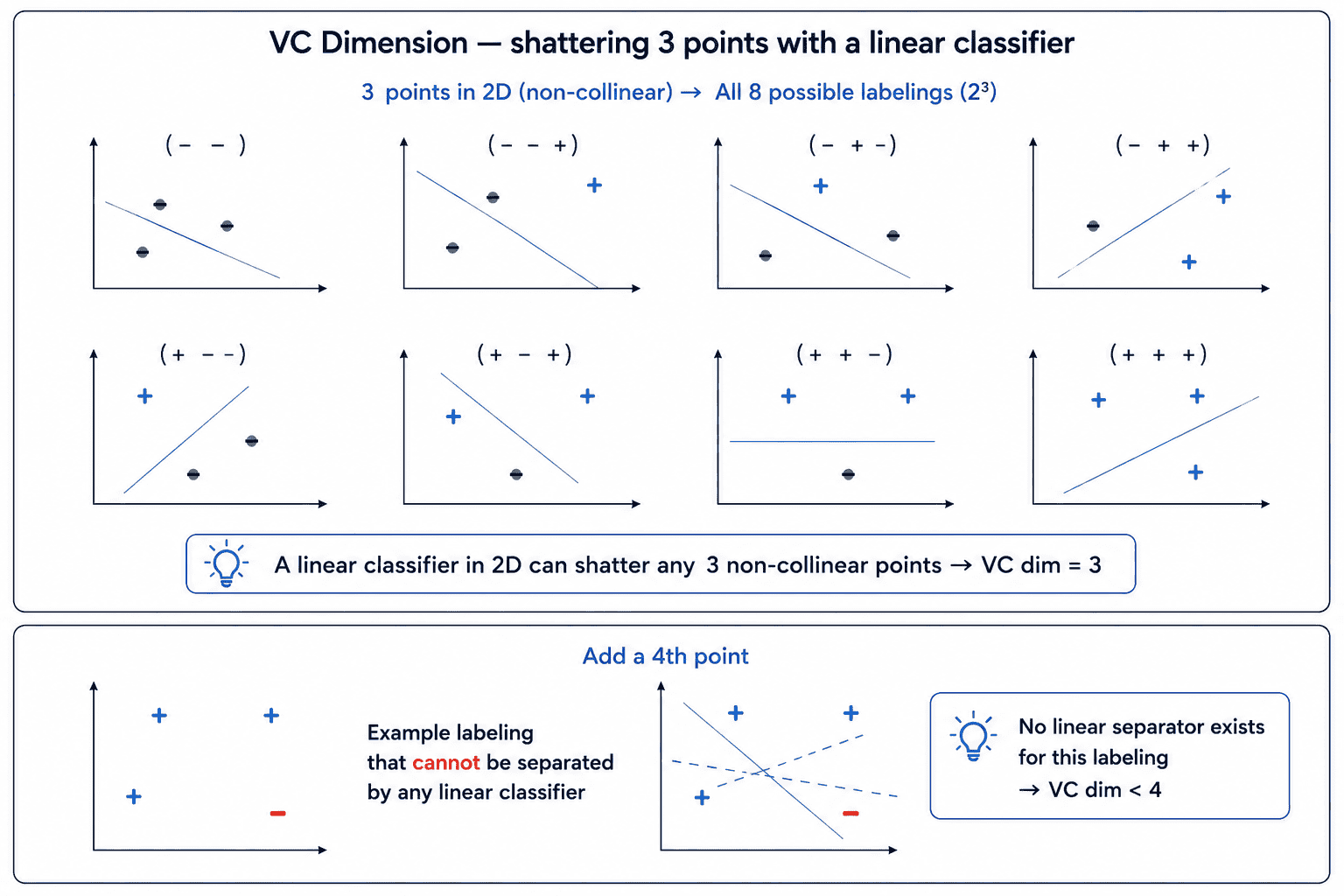
print(f"DBSCAN found {n_clusters} clusters, {n_outliers} outliers")The Vapnik-Chervonenkis (VC) dimension is a measure of the capacity (expressive power) of a statistical classification algorithm.
Key Insights:
- Definition: It is defined as the maximum number of points that can be 'shattered' (correctly classified for any label assignment) by the algorithm.
- Generalization: A model with a high VC dimension can learn more complex patterns but is at greater risk of overfitting.
- Theory: Statistical learning theory uses VC dimension to provide bounds on the difference between training error and true test error.
SHAP (SHapley Additive exPlanations) is a game-theoretic approach to explain the output of any machine learning model.
How it works:
- Shapley Values: It calculates the contribution of each feature to a prediction by averaging its marginal contribution across all possible feature combinations.
- Consistency: If a model changes so that a feature's contribution increases, its SHAP value will not decrease.
Interpretation:
- Positive SHAP value: The feature pushes the prediction higher than the average baseline.
- Negative SHAP value: The feature pushes the prediction lower than the average baseline.
import shap
import xgboost as xgb

model = xgb.XGBClassifier().fit(X_train, y_train)

# TreeSHAP — exact, fast for tree-based models
explainer   = shap.TreeExplainer(model)
shap_values = explainer(X_test)   # shape: (n_samples, n_features)

# 1. Global feature importance — mean |SHAP| across all samples
shap.plots.bar(shap_values)

# 2. Beeswarm — distribution of SHAP values per feature (best global view)
shap.plots.beeswarm(shap_values)

# 3. Waterfall — explain one specific prediction
shap.plots.waterfall(shap_values[0])         # why did sample 0 get this prediction?

# 4. Dependence plot — feature value vs SHAP + interaction coloring
shap.plots.scatter(shap_values[:, "age"], color=shap_values[:, "income"])

# For non-tree models (neural nets, etc.) — use KernelSHAP (slower)
background  = shap.maskers.Independent(X_train, max_samples=100)
explainer2  = shap.Explainer(sklearn_model, background)
shap_values2= explainer2(X_test[:50])

# Interpret: SHAP > 0 → feature pushed prediction above baseline
#            SHAP < 0 → feature pushed prediction below baseline
# Baseline = E[f(X)] across training dataBayesian optimization is a strategy for finding the global optimum of an expensive-to-evaluate black-box function (like the accuracy of a deep neural network).
Process:
1. Surrogate Model: It builds a probabilistic model (e.g., Gaussian Process) of the objective function.
2. Acquisition Function: It uses an acquisition function (e.g., Expected Improvement) to decide which set of hyperparameters to test next.
Advantages:
- Efficiency: Finds better hyperparameters in far fewer iterations than random or grid search.
- Balancing: Automatically balances exploration (trying new areas) and exploitation (refining known good areas).
import optuna
from sklearn.ensemble import RandomForestClassifier
from sklearn.model_selection import cross_val_score

# Optuna uses TPE (Tree-Structured Parzen Estimator) — Bayesian optimisation
def objective(trial):
    params = {
        "n_estimators":     trial.suggest_int("n_estimators", 50, 500),
        "max_depth":        trial.suggest_int("max_depth", 2, 20),
        "min_samples_leaf": trial.suggest_int("min_samples_leaf", 1, 20),
        "max_features":     trial.suggest_categorical("max_features", ["sqrt", "log2", None]),
        "class_weight":     trial.suggest_categorical("class_weight", ["balanced", None]),
    }
    rf = RandomForestClassifier(**params, random_state=42, n_jobs=-1)
    scores = cross_val_score(rf, X_train, y_train, cv=5, scoring="roc_auc")
    return scores.mean()

study = optuna.create_study(
    direction="maximize",
    sampler=optuna.samplers.TPESampler(seed=42),
    pruner=optuna.pruners.MedianPruner(n_warmup_steps=5),
)
study.optimize(objective, n_trials=100, n_jobs=1)
print(f"Best AUC: {study.best_value:.4f}")
print(f"Best params: {study.best_params}")

# Visualise
optuna.visualization.plot_param_importances(study).show()
optuna.visualization.plot_optimization_history(study).show()While predictive ML answers 'What will happen?', causal inference answers 'What if I do X?'. It aims to understand the cause-and-effect relationship rather than just correlations.
Key Differences:
- Predictive ML: Learns associations P(y|x). If I see a rainy day, I expect people to carry umbrellas.
- Causal Inference: Learns interventions P(y | do(x)). If I force people to carry umbrellas, will it rain?
Challenges:
- Confounders: Variables that affect both the treatment and the outcome, creating a false correlation.
- Counterfactuals: We can never observe what would have happened to the same person if they hadn't received a treatment.
| Property | Predictive ML | Causal Inference |
|---|---|---|
| Core question | What will happen? (P(y|x)) | What if I do X? (P(y | do(x))) |
| Learns | Correlations and associations | Cause-and-effect relationships |
| Sensitive to confounders | No — exploits all signals | Yes — must control for them |
| Gold standard | Held-out test set | Randomised A/B experiment |
| Observational data OK? | Yes | Requires careful design (IV, DiD, DML) |
| Tools | XGBoost, LightGBM, Neural Nets | DoWhy, EconML, CausalForest |
Key differences between predictive machine learning and causal inference.
# Double ML (Chernozhukov et al.) — causal effect estimation
# Goal: estimate effect of treatment T on outcome Y, controlling for X (confounders)
from econml.dml import LinearDML, CausalForestDML
from sklearn.ensemble import GradientBoostingRegressor, GradientBoostingClassifier

# LinearDML — assumes linear treatment effect
dml = LinearDML(
    model_y=GradientBoostingRegressor(),   # predict outcome from controls
    model_t=GradientBoostingClassifier(),  # predict treatment from controls
    cv=5,
    random_state=42,
)
dml.fit(Y=y, T=treatment, X=X_effect_modifiers, W=X_controls)

# Average treatment effect (ATE)
print(f"ATE: {dml.ate(X):.4f}")

# Heterogeneous treatment effects — effect varies by individual
ate_lb, ate_ub = dml.ate_interval(X, alpha=0.05)
print(f"95% CI: [{ate_lb:.4f}, {ate_ub:.4f}]")

# CausalForest — fully non-parametric heterogeneous effects
cf = CausalForestDML(model_y=GradientBoostingRegressor(),
                     model_t=GradientBoostingClassifier(), cv=5)
cf.fit(y, treatment, X=X_effect, W=X_control)
CATE = cf.effect(X_test) # individual-level treatment effectsMissing data can be categorized based on the mechanism of missingness, which dictates the best strategy for handling it.
Mechanisms:
- MCAR (Missing Completely at Random): No relationship between the missingness and any data.
- MAR (Missing at Random): Missingness is related to observed data but not the missing values themselves.
- MNAR (Missing Not at Random): Missingness depends on the values that are missing.
Strategies:
- Simple Imputation: Filling with mean, median, or mode (best for MCAR).
- Advanced Imputation: KNN or MICE (Iterative Imputer).
- Model-Native handling: Some algorithms (like XGBoost) can learn the best direction for missing values during training.
import pandas as pd
import numpy as np
from sklearn.impute import SimpleImputer, KNNImputer
from sklearn.experimental import enable_iterative_imputer  # noqa
from sklearn.impute import IterativeImputer
from sklearn.pipeline import Pipeline

# First: diagnose missingness
print(df.isnull().mean().sort_values(ascending=False))   # % missing per column

# ── Simple Imputation (fast baseline) ──────────────────────────────
num_imputer  = SimpleImputer(strategy='median')   # robust to outliers
cat_imputer  = SimpleImputer(strategy='most_frequent')

# ── Add missingness indicator (preserve information) ──────────────
for col in df.columns[df.isnull().any()]:
    df[f"{col}_was_missing"] = df[col].isnull().astype(int)

# ── KNN Imputation (uses similar rows) ────────────────────────────
knn_imputer = KNNImputer(n_neighbors=5, weights='distance')
X_imputed   = knn_imputer.fit_transform(X_train)

# ── MICE / Iterative Imputer (best for MAR) ───────────────────────
mice = IterativeImputer(
    estimator=None,     # default: BayesianRidge; can swap for RF
    max_iter=10,
    random_state=42
)
X_mice = mice.fit_transform(X_train)

# ── XGBoost/LightGBM handle NaNs natively ────────────────────────
# Just pass X with NaN values — they learn the optimal split directionLearning to Rank (LTR) is used when the goal is to produce an ordered list of items, such as in search engines or recommendation systems.
Comparison:
- Regression: Predicts a score (e.g., house price).
- Classification: Predicts a label (e.g., spam vs not spam).
- LTR: Focuses on the relative order between items.
Approaches:
- Pointwise: Treat as regression on individual items.
- Pairwise: Minimize the number of misordered pairs.
- Listwise: Optimize ranking metrics (like NDCG) directly across the entire list.
| Property | Pointwise | Pairwise | Listwise |
|---|---|---|---|
| Treats as | Regression / Classification | Binary classification on pairs | Sequence optimisation |
| Optimises | Per-item relevance score | Pairwise order correctness | Ranking metric (NDCG, MAP) |
| Considers list structure | No | Partial (pairs only) | Yes — full ranked list |
| Computational cost | Low (O(n)) | Medium (O(n²) pairs) | High (O(n log n)+) |
| Typical algorithms | RankNet pointwise mode | RankNet, RankSVM | LambdaMART, LightGBM LambdaRank |
Comparison of the three learning-to-rank paradigms: pointwise, pairwise, and listwise.
import lightgbm as lgb
import numpy as np
from sklearn.datasets import make_classification

# LambdaMART via LightGBM — native LTR support
# Dataset structure: features + relevance labels + query_group_sizes

# Example: 3 queries with 4, 3, 5 items respectively
query_sizes  = [4, 3, 5]                   # items per query
y_relevance  = np.array([3,2,1,0, 2,2,0, 3,3,2,1,0])  # 0-3 graded relevance

train_data = lgb.Dataset(
    X_train,
    label=y_relevance,
    group=query_sizes,     # CRITICAL — tells LightGBM query boundaries
)

params = {
    "objective":  "lambdarank",
    "metric":     "ndcg",              # Normalised Discounted Cumulative Gain
    "ndcg_eval_at": [1, 3, 5, 10],    # NDCG@1, @3, @5, @10
    "learning_rate": 0.05,
    "num_leaves":    127,
    "min_data_in_leaf": 1,
    "label_gain": [0, 1, 3, 7],       # gain weights for 0,1,2,3 relevance levels
}

callbacks = [lgb.early_stopping(50), lgb.log_evaluation(25)]
model = lgb.train(params, train_data, num_boost_round=500,
                  valid_sets=[val_data], callbacks=callbacks)

# Predict relevance scores → sort within each query
scores = model.predict(X_test)Conformal prediction is a framework that provides a way to quantify uncertainty with a rigorous statistical guarantee.
Key Benefits:
- Coverage Guarantee: You can specify a confidence level (e.g., 95%), and the prediction set is guaranteed to contain the true value 95% of the time.
- Distribution-Free: It makes no assumptions about the underlying distribution of the data (no 'Normal assumption').
- Model-Agnostic: It can be applied on top of any pre-trained machine learning model.
from mapie.classification import MapieClassifier
from mapie.regression    import MapieRegressor
from sklearn.ensemble    import RandomForestClassifier, RandomForestRegressor
import numpy as np

# ── Classification — prediction SETS with guaranteed coverage ────────
clf = RandomForestClassifier(n_estimators=200, random_state=42)
mapie_clf = MapieClassifier(estimator=clf, method="raps",    # RAPS: size-adaptive
                             cv="prefit")
clf.fit(X_train, y_train)
mapie_clf.fit(X_calib, y_calib)                      # calibration set (held-out)

alpha = 0.10   # target miscoverage rate → 90% coverage guarantee
y_pred, y_sets = mapie_clf.predict(X_test, alpha=alpha)
# y_sets[i] = set of labels that MUST include true label 90% of the time
print(f"Average set size: {y_sets.sum(axis=1).mean():.2f}")
print(f"Empirical coverage: {np.mean([y_test[i] in y_sets[i] for i in range(len(y_test))]):.3f}")

# ── Regression — prediction INTERVALS ────────────────────────────────
reg = RandomForestRegressor(n_estimators=200, random_state=42).fit(X_train, y_train)
mapie_reg = MapieRegressor(estimator=reg, method="plus", cv="prefit")
mapie_reg.fit(X_calib, y_calib)
y_pred, y_pis = mapie_reg.predict(X_test, alpha=0.10)
# y_pis[:, 0, 0], y_pis[:, 1, 0] = lower and upper bounds of 90% intervalA Gaussian Process (GP) is a non-parametric method that provides a way to model functions with uncertainty quantification.
Characteristics:
- Kernel-Based: The 'heart' of a GP is the kernel function, which defines the similarity between points.
- Calibrated Uncertainty: Instead of a single value, it returns a full probability distribution (mean and variance).
When to use:
- Bayesian Optimization (to find the best hyperparameters).
- Small datasets where understanding uncertainty is as important as the prediction.
- Time series or spatial modeling.
from sklearn.gaussian_process import GaussianProcessRegressor
from sklearn.gaussian_process.kernels import (
    RBF, Matern, WhiteKernel, ConstantKernel as C
)
import numpy as np

# Define kernel (covariance function)
kernel = (
    C(1.0, (1e-3, 1e3))                     # amplitude
    * RBF(length_scale=1.0, length_scale_bounds=(1e-2, 1e2))   # smoothness
    + WhiteKernel(noise_level=0.1)           # observation noise
)

gpr = GaussianProcessRegressor(
    kernel=kernel,
    n_restarts_optimizer=10,   # multiple optimisation starts for marginal likelihood
    normalize_y=True,
    random_state=42
)
gpr.fit(X_train, y_train)    # O(n³) — only feasible for n < ~5,000

# Predict with uncertainty
X_test_plot = np.linspace(-3, 3, 200).reshape(-1, 1)
y_mean, y_std = gpr.predict(X_test_plot, return_std=True)

# 95% credible interval
y_lower = y_mean - 1.96 * y_std
y_upper = y_mean + 1.96 * y_std

print(f"Learned kernel: {gpr.kernel_}")   # inspects optimised hyperparameters

# For large datasets: Sparse GPs (inducing points)
# sklearn: Use GPy or GPyTorch for sparseGP at scaleDesigning a real-time fraud detection system involves building a low-latency pipeline that can process millions of transactions while identifying suspicious patterns instantly.
Key Components:
- Low Latency Features: Using tools like Redis or Flink to compute and serve features (like txn velocity) in milliseconds.
- Model Serving: Deploying models (like XGBoost or LightGBM) as microservices with high availability.
- Calibrated Probability: Ensuring the fraud score (e.g., 0.8) actually corresponds to the likelihood (80%) to aid human review.
- Feedback Loop: A system to ingest labels from chargebacks and disputes to retrain the model regularly.

# Feature engineering for fraud — real-time aggregation window features
import redis
import time

r = redis.Redis(host='localhost', port=6379)

def get_realtime_features(card_id: str, merchant_id: str, amount: float) -> dict:
    now_ts  = int(time.time())
    hour_ts = now_ts - 3600
    day_ts  = now_ts - 86400

    # Sliding window aggregates from Redis sorted sets
    txn_1h   = r.zcount(f"card:{card_id}:txns",  hour_ts, now_ts)
    spend_1h = r.zscore(f"card:{card_id}:spend1h", card_id) or 0
    txn_1d   = r.zcount(f"card:{card_id}:txns",  day_ts,  now_ts)

    # Latest known features from feature store
    device_fp_match = r.get(f"card:{card_id}:device") == r.get("req:device")
    geo_velocity_km = float(r.get(f"card:{card_id}:geo_vel") or 0)

    return {
        "txn_count_1h":       txn_1h,
        "spend_1h":           spend_1h,
        "txn_count_24h":      txn_1d,
        "amount_zscore":      (amount - float(r.get(f"card:{card_id}:avg_amt") or amount)) /
                              max(float(r.get(f"card:{card_id}:std_amt") or 1), 1),
        "device_fp_match":    int(device_fp_match),
        "geo_velocity_km":    geo_velocity_km,
        "merchant_risk_score":float(r.get(f"merch:{merchant_id}:risk") or 0.5),
}Before reaching for complex models, establish a naive baseline (majority class, mean prediction). This anchors the conversation and shows you understand the actual problem difficulty. A random forest beating a mean prediction by 2% is not impressive; beating it by 30% is.
Never start modelling without confirming the metric. Accuracy, AUC, F1, RMSE, and NDCG lead to very different model choices and thresholds. The business metric (revenue impact, churn reduction) should also be mapped to a model metric so you can justify your choices.
Interviewers test whether you know when to stop chasing performance. A logistic regression at 0.82 AUC that's interpretable, fast, and explainable to regulators is often more valuable in production than a neural network at 0.85 AUC that's a black box. Always discuss interpretability, latency, and maintenance costs alongside accuracy.
ML system design interviews expect you to think beyond model training. Mention feature stores, model registries, drift monitoring, shadow deployment, and retraining pipelines. Candidates who only talk about model accuracy and skip infrastructure are seen as junior regardless of their algorithm knowledge.
Machine learning interviews reward engineers who combine theoretical rigour with practical judgment. The most successful candidates don't just know the formulas — they know when to apply each technique, how to evaluate it fairly, and how to deploy it reliably in production. These 25 questions will sharpen all three dimensions.
Build a portfolio project end-to-end: raw data → feature engineering → model selection with CV → hyperparameter tuning → inference API → monitoring dashboard. Walking through that project in detail is worth ten textbook recitations. Good luck!
Explore more resources →Md Rashid
Software engineer and career coach with 6+ years in the tech industry. Writes about interview prep, developer careers, and tech job markets.

Top 25 AI Engineer Interview Questions and Answers (2026 Edition)
Ace your next AI engineer interview with this comprehensive guide covering LLMs, transformers, RAG, fine-tuning, RLHF, diffusion models, AI safety, and production ML systems.

The Complete Linux Commands Cheat Sheet 2026
Every essential Linux command defined with clean, practical examples. Covers file navigation, system monitoring, user permissions, networking, package management, and shell scripting.

The Complete JavaScript Cheat Sheet 2026
Every essential JavaScript syntax, method, and pattern you need — from variables, arrays, and objects to async/await, closures, ES2026 features, and DOM manipulation. Clean, copy-paste-ready examples.
The Complete SQL Cheat Sheet 2026
Every SQL command, function, and pattern you need — from basic SELECT queries to advanced window functions, CTEs, indexes, and transactions. Clean, runnable examples for PostgreSQL, MySQL, and SQL Server.