
Ace your next database or backend interview with this comprehensive guide covering joins, CTEs, window functions, normalization, and advanced performance optimization techniques.
SQL (Structured Query Language) is the standard language for interacting with relational database management systems (RDBMs).
Main Purposes:
- Data Definition: Creating and modifying the structure (schema) of tables and databases.
- Data Manipulation: Inserting, updating, and deleting records within tables.
- Data Querying: Retrieving specific information based on complex filters and conditions.
- Data Control: Managing user permissions and security to ensure data integrity.
SQL commands are categorized based on their function within the database lifecycle.
Core Categories:
- DDL (Data Definition Language): Commands that define the schema (e.g., CREATE, ALTER, DROP).
- DML (Data Manipulation Language): Commands that modify the actual data (e.g., INSERT, UPDATE, DELETE).
- DQL (Data Query Language): The primary command used for info retrieval (e.g., SELECT).
- DCL (Data Control Language): Commands for security and permissions (e.g., GRANT, REVOKE).
- TCL (Transaction Control Language): Commands for managing transactions (e.g., COMMIT, ROLLBACK).
-- DDL  (schema)
CREATE TABLE employees (id INT PRIMARY KEY, name VARCHAR(100));
ALTER TABLE employees ADD COLUMN salary DECIMAL(10,2);
DROP TABLE employees;

-- DML  (data)
INSERT INTO employees VALUES (1, 'Alice', 80000);
UPDATE employees SET salary = 85000 WHERE id = 1;
DELETE FROM employees WHERE id = 1;

-- DQL  (query)
SELECT * FROM employees WHERE salary > 70000;

-- DCL  (permissions)
GRANT SELECT ON employees TO hr_user;
REVOKE SELECT ON employees FROM hr_user;

-- TCL  (transactions)
BEGIN; COMMIT; ROLLBACK; SAVEPOINT sp1;While both are used for filtering, they operate at different stages of the SQL execution pipeline.
Key Differences:
- Execution Level: WHERE filters individual rows from the source; HAVING filters grouped results after aggregation.
- Aggregate Functions: You cannot use aggregates (like SUM or AVG) in a WHERE clause; you must use HAVING for that.
- Best Practice: Use WHERE to reduce the number of rows as early as possible before grouping to improve performance.
-- WHERE filters raw rows before aggregation
SELECT department, COUNT(*) AS headcount
FROM employees
WHERE salary > 50000          -- filter rows first
GROUP BY department;

-- HAVING filters aggregated groups
SELECT department, AVG(salary) AS avg_sal
FROM employees
GROUP BY department
HAVING AVG(salary) > 70000;   -- filter after grouping

-- Both together
SELECT department, SUM(salary) AS total_payout
FROM employees
WHERE active = TRUE            -- only active employees
GROUP BY department
HAVING SUM(salary) > 500000; -- departments spending > 500kJOINs allow you to combine and relate data across multiple tables based on a shared column.
Main Join Types:
- INNER JOIN: Returns only the records where there is a match in both tables.
- LEFT (OUTER) JOIN: Returns all records from the left table, and matching records from the right (NULLs if no match).
- RIGHT (OUTER) JOIN: Returns all records from the right table, and matching records from the left.
- FULL (OUTER) JOIN: Returns all records when there is a match in either the left or right table.
- CROSS JOIN: Returns the Cartesian product (every combination of rows) of both tables.
-- INNER JOIN — only matching rows
SELECT e.name, d.dept_name
FROM employees e
INNER JOIN departments d ON e.dept_id = d.id;

-- LEFT JOIN — all employees, NULLs if no department
SELECT e.name, d.dept_name
FROM employees e
LEFT JOIN departments d ON e.dept_id = d.id;

-- FULL OUTER JOIN — all rows from both tables
SELECT e.name, d.dept_name
FROM employees e
FULL OUTER JOIN departments d ON e.dept_id = d.id;

-- SELF JOIN — find employees and their managers
SELECT e.name AS employee, m.name AS manager
FROM employees e
LEFT JOIN employees m ON e.manager_id = m.id;Both constraints ensure data uniqueness in a column, but they serve slightly different architectural roles.
Main Differences:
- Nullability: A PRIMARY KEY cannot contain NULL values; a UNIQUE KEY typically allows one NULL value.
- Quantity: A table can have only one PRIMARY KEY, but it can have multiple UNIQUE keys.
- Purpose: The PRIMARY KEY is the 'official' unique identifier for a row, whereas UNIQUE keys are used for auxiliary unique fields like email or phone.
CREATE TABLE users (
  id         INT          PRIMARY KEY,       -- NOT NULL, unique, only one
  email      VARCHAR(255) UNIQUE,            -- unique, allows one NULL, multiple allowed
  phone      VARCHAR(20)  UNIQUE,
  username   VARCHAR(50)  NOT NULL
);

-- Composite Primary Key
CREATE TABLE order_items (
  order_id   INT,
  product_id INT,
  quantity   INT,
  PRIMARY KEY (order_id, product_id)         -- combination must be unique
);A FOREIGN KEY creates a logical link between two tables, ensuring that the data in one table matches the data in another.
Key Concepts:
- Parent vs. Child: The table with the PRIMARY KEY is the 'parent'; the table containing the FOREIGN KEY is the 'child'.
- Referential Integrity: A set of rules that prevent 'orphan rows' (child rows referencing a non-existent parent).
- Actions: You can define what happens to child rows when a parent is deleted (e.g., CASCADE, SET NULL).
CREATE TABLE departments (
  id   INT PRIMARY KEY,
  name VARCHAR(100) NOT NULL
);

CREATE TABLE employees (
  id      INT PRIMARY KEY,
  name    VARCHAR(100),
  dept_id INT,
  FOREIGN KEY (dept_id) REFERENCES departments(id)
    ON DELETE SET NULL    -- if dept deleted, set NULL
    ON UPDATE CASCADE     -- if dept id changes, propagate
);

-- This will FAIL if dept_id=99 doesn't exist in departments
INSERT INTO employees (id, name, dept_id) VALUES (1, 'Alice', 99); -- ❌Both operators are used to combine the result sets of two or more SELECT statements into a single output.
Key Differences:
- Deduplication: UNION performs a distinct sort to remove duplicate rows, whereas UNION ALL keeps all rows.
- Efficiency: UNION ALL is significantly faster because it doesn't need to check for duplicates or perform sorting.
- Result Set: Use UNION only when you explicitly need a unique set of records; otherwise, default to UNION ALL for performance.
-- UNION — removes duplicates (slower)
SELECT city FROM customers
UNION
SELECT city FROM suppliers;

-- UNION ALL — keeps all rows including duplicates (faster)
SELECT city FROM customers
UNION ALL
SELECT city FROM suppliers;

-- Requirements: same number of columns, compatible data types
-- Column names in result come from the first SELECTAggregate functions perform a calculation on a set of values and return a single summarizing value.
Common Aggregates:
- COUNT: Returns the total number of rows or non-null values.
- SUM: Returns the total mathematical sum of a numeric column.
- AVG: Returns the average value of a numeric column.
- MIN/MAX: Returns the smallest or largest value in a set.
- Grouping: These are almost always used in conjunction with the GROUP BY clause to summarize data by category.
SELECT
  department,
  COUNT(*)          AS headcount,
  SUM(salary)       AS total_payroll,
  AVG(salary)       AS avg_salary,
  MIN(salary)       AS lowest_salary,
  MAX(salary)       AS highest_salary
FROM employees
GROUP BY department
ORDER BY total_payroll DESC;

-- COUNT(*) vs COUNT(column)
SELECT
  COUNT(*)        AS total_rows,       -- counts all rows incl. NULLs
  COUNT(manager)  AS rows_with_manager -- excludes NULL managers
FROM employees;SQL is written in one order but processed by the database engine in another. Understanding this logic is vital for troubleshooting errors.
Logical Processing Order:
1. FROM / JOIN: Identifying the base tables and combining them.
2. WHERE: Filtering the raw data rows.
3. GROUP BY: Organizing rows into groups based on specified columns.
4. HAVING: Filtering the grouped data.
5. SELECT: Choosing which columns and expressions to return.
6. ORDER BY: Sorting the final result set.
7. LIMIT / OFFSET: Paginating the results.
-- Writing order:
-- SELECT → FROM → WHERE → GROUP BY → HAVING → ORDER BY → LIMIT

-- Execution order:
-- 1. FROM / JOIN  — identify the data source and join tables
-- 2. WHERE        — filter individual rows
-- 3. GROUP BY     — group remaining rows
-- 4. HAVING       — filter groups
-- 5. SELECT       — choose columns and evaluate expressions
-- 6. DISTINCT     — remove duplicates
-- 7. ORDER BY     — sort results (can use SELECT aliases here)
-- 8. LIMIT/OFFSET — paginate

-- Example: This fails because alias defined in SELECT (#5)
--          cannot be referenced in WHERE (#2)
SELECT salary * 1.1 AS raise
FROM employees
WHERE raise > 60000;    -- ❌ ERROR: column "raise" doesn't exist

-- Fix: repeat the expression or use a subquery / CTE
SELECT salary * 1.1 AS raise
FROM employees
WHERE salary * 1.1 > 60000; -- ✅While both might appear 'blank', they have completely different meanings in relational database theory.
Key Concepts:
- NULL: Represents 'No Value' or 'Unknown'. It indicates data is missing or not applicable.
- Empty String: Represents a known, defined value (a string with 0 length). It's like an empty bucket, whereas NULL is the absence of a bucket.
- Comparison: NULL cannot be compared using `=` (you must use `IS NULL`). Empty strings can be compared directly.
-- Checking for NULL — must use IS NULL / IS NOT NULL
SELECT * FROM users WHERE phone IS NULL;      -- ✅
SELECT * FROM users WHERE phone = NULL;       -- ❌ always false!

-- Checking for empty string
SELECT * FROM users WHERE phone = '';         -- ✅

-- NULL in expressions always yields NULL
SELECT NULL + 100;      -- NULL
SELECT NULL = NULL;     -- NULL (not TRUE!)
SELECT NULL IS NULL;    -- TRUE

-- COALESCE — returns first non-NULL value
SELECT COALESCE(phone, 'Not provided') FROM users;

-- NULLIF — returns NULL if two values are equal
SELECT NULLIF(salary, 0) FROM employees; -- treats 0 as NULLA subquery is a SQL query nested inside another query, typically within the WHERE, FROM, or SELECT clauses.
Main Subquery Types:
- Scalar Subquery: Returns a single value (one row, one column). Useful for comparisons.
- Row Subquery: Returns a single row with multiple columns.
- Table/Multiple-Row Subquery: Returns multiple rows (e.g., used with the `IN` or `EXISTS` operators).
- Correlated Subquery: A subquery that depends on values from the outer query, executing once for every row processed by the outer query.
-- Scalar subquery (returns 1 value)
SELECT name, salary,
  (SELECT AVG(salary) FROM employees) AS company_avg
FROM employees;

-- IN subquery (returns a list)
SELECT name FROM employees
WHERE dept_id IN (
  SELECT id FROM departments WHERE location = 'NYC'
);

-- EXISTS (correlated — references outer query)
SELECT * FROM customers c
WHERE EXISTS (
  SELECT 1 FROM orders o WHERE o.customer_id = c.id
);

-- FROM subquery (inline view / derived table)
SELECT dept, avg_sal
FROM (
  SELECT department AS dept, AVG(salary) AS avg_sal
  FROM employees
  GROUP BY department
) AS dept_stats
WHERE avg_sal > 70000;A Common Table Expression (CTE) is a temporary result set that you can reference within a SELECT, INSERT, UPDATE, or DELETE statement.
Key Advantages:
- Better Readability: They let you break complex, deeply nested subqueries into logical, named blocks.
- Reusability: You can reference the same CTE multiple times within a single query.
- Recursion: Recursive CTEs are the only way in SQL to traverse hierarchical data (like org charts or file systems).
- Scope: They only exist for the duration of the query, avoiding schema clutter.
-- Basic CTE
WITH high_earners AS (
  SELECT id, name, salary, department
  FROM employees
  WHERE salary > 90000
)
SELECT department, COUNT(*) AS top_employees
FROM high_earners
GROUP BY department;

-- Multiple CTEs chained
WITH dept_avg AS (
  SELECT department, AVG(salary) AS avg_sal
  FROM employees
  GROUP BY department
),
above_avg AS (
  SELECT e.name, e.salary, d.avg_sal
  FROM employees e
  JOIN dept_avg d ON e.department = d.department
  WHERE e.salary > d.avg_sal
)
SELECT * FROM above_avg ORDER BY salary DESC;

-- Recursive CTE — employee hierarchy
WITH RECURSIVE org_chart AS (
  SELECT id, name, manager_id, 1 AS level
  FROM employees WHERE manager_id IS NULL          -- root
  UNION ALL
  SELECT e.id, e.name, e.manager_id, o.level + 1
  FROM employees e
  JOIN org_chart o ON e.manager_id = o.id          -- recurse
)
SELECT * FROM org_chart ORDER BY level;Window functions perform a calculation across a set of table rows that are somehow related to the current row.
Core Mechanisms:
- OVER Clause: Defines the 'window' of rows the function operates on.
- PARTITION BY: Divides the rows into groups (similar to GROUP BY, but rows remain un-collapsed).
- ORDER BY: Specifies the sequence of rows within each partition.
- Benefits: They allow you to perform complex analytics like running totals, rankings, and moving averages without complex self-joins.
-- ROW_NUMBER, RANK, DENSE_RANK
SELECT
  name, department, salary,
  ROW_NUMBER() OVER (PARTITION BY department ORDER BY salary DESC) AS row_num,
  RANK()       OVER (PARTITION BY department ORDER BY salary DESC) AS rank,
  DENSE_RANK() OVER (PARTITION BY department ORDER BY salary DESC) AS dense_rank
FROM employees;

-- Running total (SUM with frame)
SELECT
  order_date, amount,
  SUM(amount) OVER (ORDER BY order_date
    ROWS BETWEEN UNBOUNDED PRECEDING AND CURRENT ROW) AS running_total
FROM orders;

-- LAG / LEAD — access adjacent rows
SELECT
  month, revenue,
  LAG(revenue, 1) OVER (ORDER BY month)  AS prev_month,
  revenue - LAG(revenue, 1) OVER (ORDER BY month) AS delta
FROM monthly_revenue;

-- NTILE — divide into N buckets
SELECT name, salary,
  NTILE(4) OVER (ORDER BY salary) AS salary_quartile
FROM employees;An index is a powerful data structure that improves the speed of data retrieval operations on a database table at the cost of slower writes.
How it works:
- B-Tree Structure: Most indexes use a balanced tree to allow the database to find specific rows in logarithmic time instead of scanning the whole table.
- Pointers: The index contains the values from the indexed columns and 'pointers' to the physical location of the rest of the row data.
- Selective Indexing: You should index columns frequently used in `WHERE`, `JOIN`, and `ORDER BY` clauses to maximize performance gains.
-- Create a simple index
CREATE INDEX idx_employees_dept ON employees(department);

-- Composite index (order matters!)
CREATE INDEX idx_emp_dept_salary ON employees(department, salary);

-- Unique index
CREATE UNIQUE INDEX idx_users_email ON users(email);

-- Partial index — only index subset of rows
CREATE INDEX idx_active_users ON users(email) WHERE active = TRUE;

-- Check index usage with EXPLAIN
EXPLAIN ANALYZE
SELECT * FROM employees WHERE department = 'Engineering';
-- Look for "Index Scan" vs "Seq Scan"

-- Covering index — all required columns are in the index
CREATE INDEX idx_covering ON employees(department, salary, name);
SELECT name, salary FROM employees WHERE department = 'Engineering';
-- Above uses index only scan — no table access neededA transaction is a single logic unit of work that contains one or more SQL statements.
ACID Guarantees:
- Atomicity: 'All or nothing'. If one statement fails, the entire transaction is rolled back.
- Consistency: Transactions always move the database from one valid state to another, following all rules and constraints.
- Isolation: Concurrent transactions are processed independently and do not interfere with each other.
- Durability: Once a transaction is committed, the changes are permanent and survive system crashes.
-- BEGIN TRANSACTION; (SQL Server)
-- PostgreSQL/MySQL use: BEGIN; or START TRANSACTION;
BEGIN TRANSACTION;

  UPDATE accounts SET balance = balance - 500
  WHERE account_id = 'A';   -- debit sender

  UPDATE accounts SET balance = balance + 500
  WHERE account_id = 'B';   -- credit receiver

COMMIT;   -- both succeed → persisted

-- If any error occurs:
ROLLBACK; -- both changes are undone atomically

-- SAVEPOINT for partial rollback
BEGIN;
  INSERT INTO orders VALUES (101, 'Alice');
  SAVEPOINT after_order;

  INSERT INTO order_items VALUES (101, 'Widget', 2);
  -- If this fails:
  ROLLBACK TO SAVEPOINT after_order;  -- keep the order, undo items

COMMIT;Isolation levels define the degree to which a transaction must be isolated from data modifications made by other concurrent transactions.
The Standard Levels:
- READ UNCOMMITTED: Lowest level. Allows 'dirty reads' where a transaction can see uncommitted data from others.
- READ COMMITTED: Standard for many DBs. Guarantees that any data read is committed at the moment it is read.
- REPEATABLE READ: Ensures that if you read the same data twice in one transaction, the values will be identical.
- SERIALIZABLE: Highest level. Transactions are executed in a way that is equivalent to them running one after another.
-- Set isolation level (PostgreSQL/Standard)
SET TRANSACTION ISOLATION LEVEL READ COMMITTED;

-- READ UNCOMMITTED — can see uncommitted "dirty" data (rarely used)
-- READ COMMITTED   — only sees committed data (default in many DBs)
-- REPEATABLE READ  — same query returns same rows within transaction
-- SERIALIZABLE     — highest isolation, transactions appear sequential

-- Isolation level problems:
-- ┌──────────────────────┬───────────┬─────────────┬───────────────┐
-- │ Level                │ Dirty Read│ Non-Repeat. │ Phantom Read  │
-- ├──────────────────────┼───────────┼─────────────┼───────────────┤
-- │ READ UNCOMMITTED     │    ✅     │    ✅       │     ✅        │
-- │ READ COMMITTED       │    ❌     │    ✅       │     ✅        │
-- │ REPEATABLE READ      │    ❌     │    ❌       │     ✅        │
-- │ SERIALIZABLE         │    ❌     │    ❌       │     ❌        │
-- └──────────────────────┴───────────┴─────────────┴───────────────┘

-- Phantom Read example:
-- T1 reads: SELECT * WHERE salary > 50k → 10 rows
-- T2 inserts a new row where salary = 80k and commits
-- T1 reads again: SELECT * WHERE salary > 50k → 11 rows (phantom!)Normalization is the technical process of organizing database columns and tables to minimize redundancy and dependency.
Core Normal Forms:
- 1NF (First Normal Form): Data is atomic (no lists in cells) and each row is unique.
- 2NF (Second Normal Form): Meets 1NF and all non-key columns depend on the entire primary key.
- 3NF (Third Normal Form): Meets 2NF and no non-key column depends on another non-key column (no transitive dependencies).
- Goal: To ensure data integrity and make the database easier to maintain and extend.
-- ❌ Unnormalized (0NF) — repeated groups
-- order_id | customer | items (comma-separated)
-- 1        | Alice    | Widget,Gadget,Donut

-- ❌ 1NF violation — non-atomic values fixed
-- order_id | customer | item
-- 1        | Alice    | Widget
-- 1        | Alice    | Gadget  ← customer redundant

-- ❌ 2NF violation — partial dependency
-- order_id | item_id | customer | item_price
-- 'customer' depends on order_id alone (not full PK)

-- ✅ 2NF — separate orders and items tables
-- orders: (order_id, customer_id)
-- order_items: (order_id, item_id, quantity)

-- ❌ 3NF violation — transitive dependency
-- employee_id | dept_id | dept_location
-- dept_location depends on dept_id, not employee_id

-- ✅ 3NF fix — separate departments table
-- employees: (employee_id, dept_id)
-- departments: (dept_id, dept_name, location)While both are blocks of reusable SQL code, they serve different purposes within a database environment.
Key Differences:
- Usage: Procedures are 'called' (e.g., `CALL proc()`); Functions are used within queries (e.g., `SELECT func()`).
- Return Value: Functions MUST return a value; Procedures may or may not return values via output parameters.
- Side Effects: Procedures can perform DML operations (INSERT/UPDATE); Functions are generally restricted to read-only logic in many systems.
- Transactions: Procedures can often manage their own transactions (COMMIT/ROLLBACK); Functions typically cannot.
-- Stored Procedure (PostgreSQL syntax — syntax differs significantly in MySQL/T-SQL)
CREATE OR REPLACE PROCEDURE transfer_funds(
  sender_id INT,
  receiver_id INT,
  amount DECIMAL
)
LANGUAGE plpgsql AS $$
BEGIN
  UPDATE accounts SET balance = balance - amount
  WHERE id = sender_id;

  UPDATE accounts SET balance = balance + amount
  WHERE id = receiver_id;

  INSERT INTO transfer_log VALUES (sender_id, receiver_id, amount, NOW());
  COMMIT;
END;
$$;

-- Call it
CALL transfer_funds(1, 2, 500.00);

-- Function — returns a value, used inline
CREATE OR REPLACE FUNCTION get_salary_grade(sal DECIMAL)
RETURNS VARCHAR AS $$
BEGIN
  IF sal > 100000 THEN RETURN 'Senior';
  ELSIF sal > 60000 THEN RETURN 'Mid';
  ELSE RETURN 'Junior';
  END IF;
END;
$$ LANGUAGE plpgsql;

SELECT name, get_salary_grade(salary) AS grade FROM employees;A VIEW is essentially a 'stored query' that presents data from one or more tables as if it were its own table.
When to Use Views:
- Simplicity: To hide complex JOINs and calculations from the end user or application.
- Security: To grant users access to a subset of columns (excluding sensitive data like passwords).
- Consistency: To provide a stable interface even if the underlying table schemas change.
- Logic Centralization: To ensure that complex business logic is defined in one place rather than duplicated in app code.
-- Create a view (a saved query)
CREATE VIEW active_employees AS
SELECT id, name, department, salary
FROM employees
WHERE active = TRUE AND left_date IS NULL;

-- Query it like a regular table
SELECT * FROM active_employees WHERE department = 'Engineering';

-- Updatable view (simple cases only)
UPDATE active_employees SET salary = 90000 WHERE id = 42;

-- SECURITY — hide sensitive columns
CREATE VIEW employee_public_info AS
SELECT id, name, department     -- no salary, SSN
FROM employees;

GRANT SELECT ON employee_public_info TO junior_staff;

-- Materialized View (PostgreSQL, Oracle) — stores the result
CREATE MATERIALIZED VIEW monthly_sales AS
SELECT DATE_TRUNC('month', order_date) AS month, SUM(amount) AS total
FROM orders
GROUP BY 1;

REFRESH MATERIALIZED VIEW monthly_sales; -- update the cached dataDeduplication is a common data cleaning task that relies on grouping data and analyzing the frequency of occurrences.
Common Methods:
- Group By + Having: The most straightforward way. Group by all relevant columns and filter for `COUNT(*) > 1`.
- Window Functions: Using `ROW_NUMBER()` is more flexible, especially when you need to decide which specific duplicate to keep (e.g., the oldest or the newest).
- Self Joins: Joining a table to itself to find rows with matching values but different IDs.
-- Find duplicate emails
SELECT email, COUNT(*) AS occurrences
FROM users
GROUP BY email
HAVING COUNT(*) > 1
ORDER BY occurrences DESC;

-- Get the full rows for duplicates
SELECT *
FROM users
WHERE email IN (
  SELECT email
  FROM users
  GROUP BY email
  HAVING COUNT(*) > 1
);

-- Delete duplicates, keeping the row with the lowest id
DELETE FROM users
WHERE id NOT IN (
  SELECT MIN(id)
  FROM users
  GROUP BY email     -- keep the earliest duplicate per email
);

-- Using ROW_NUMBER (cleaner, modern approach)
WITH duplicates AS (
  SELECT id, ROW_NUMBER() OVER (PARTITION BY email ORDER BY id) AS rn
  FROM users
)
DELETE FROM users WHERE id IN (
  SELECT id FROM duplicates WHERE rn > 1   -- delete all but the first
);This question tests your ability to solve a classic problem using multiple logical approaches without relying on simple vendor-specific syntax like `LIMIT` or `TOP`.
Recommended Approaches:
- Window Functions: Use `DENSE_RANK()` to handle ties gracefully. It assigns the same rank to identical salaries without skipping numbers.
- Correlated Subqueries: A standard SQL approach where you find a salary such that exactly (N-1) distinct salaries are greater than it.
- Joins: You can join the table to itself and count the distinct salaries that are greater than or equal to the current row's salary.
-- Method 1: DENSE_RANK (recommended — handles ties)
SELECT DISTINCT salary
FROM (
  SELECT salary,
    DENSE_RANK() OVER (ORDER BY salary DESC) AS rnk
  FROM employees
) ranked
WHERE rnk = 3;   -- 3rd highest; change N here

-- Method 2: Correlated subquery (classic approach)
-- Find salary where exactly (N-1) distinct salaries are greater
SELECT DISTINCT salary
FROM employees e1
WHERE 2 = (            -- N-1 = 2 for 3rd highest
  SELECT COUNT(DISTINCT salary)
  FROM employees e2
  WHERE e2.salary > e1.salary
);

-- Method 3: OFFSET (simple but varies by DB)
SELECT DISTINCT salary
FROM employees
ORDER BY salary DESC
LIMIT 1 OFFSET 2;    -- skip top 2, take next = 3rd highest

-- Full row for the employee with Nth highest salary
WITH ranked AS (
  SELECT *, DENSE_RANK() OVER (ORDER BY salary DESC) AS rnk
  FROM employees
)
SELECT name, salary, department
FROM ranked WHERE rnk = 3;Query optimization is the systematic process of reducing the execution time and resource consumption (CPU, Memory, I/O) of a SQL statement.
Key Concepts:
- EXPLAIN / EXPLAIN ANALYZE: Tools that show the execution plan chosen by the optimizer. Use 'ANALYZE' to see actual runtimes versus estimates.
- Scans vs. Lookups: Identify 'Sequential Scans' (reading the whole table) and look for opportunities to replace them with 'Index Scans'.
- Join Strategies: Understand how the DB joins data (e.g., Hash Join, Nested Loop, Merge Join) to identify bottlenecks.
- Optimization Levers: Including index creation, rewriting subqueries as joins, and keeping table statistics up to date.
-- Basic EXPLAIN
EXPLAIN SELECT * FROM employees WHERE department = 'Engineering';

-- EXPLAIN ANALYZE — actually runs the query and shows real timing
EXPLAIN ANALYZE
SELECT e.name, d.dept_name
FROM employees e
JOIN departments d ON e.dept_id = d.id
WHERE e.salary > 80000;

-- Key terms in output:
-- Seq Scan      — reading all rows (no useful index)
-- Index Scan    — using an index to find rows
-- Index Only Scan — all data comes from index (fastest)
-- Hash Join     — hashing smaller table for join lookup
-- Nested Loop   — for each row in outer, scan inner
-- Merge Join    — both sides sorted, merge together
-- cost=X..Y     — estimated rows and time
-- actual time   — real elapsed time (with ANALYZE)
-- rows          — estimated vs actual row count

-- Common optimization moves:
-- 1. Add missing index on WHERE / JOIN column
-- 2. Use covering index (include all selected columns)
-- 3. Rewrite correlated subquery as JOIN / CTE
-- 4. Avoid SELECT * — project only needed columns
-- 5. Avoid functions on indexed columns in WHERE
--    WHERE UPPER(email) = 'test@example.com' ← kills index
-- WHERE email = LOWER('test@Example.com') ← index usableThe distinction between these index types lies in how the database physically stores the row data relative to the index structure.
Main Differences:
- Physical Storage: A clustered index defines the actual physical order of rows on disk. A non-clustered index is a separate structure that points to the actual data.
- Quantity: You can have only one clustered index per table (since data can only be sorted in one way), but many non-clustered indexes.
- Performance: Clustered indexes are exceptionally fast for range scans; non-clustered indexes are great for specific lookups but may require 'bookmark lookups' to retrieve the full row.
-- In SQL Server / MySQL InnoDB:
-- The PRIMARY KEY automatically becomes the clustered index.
-- All non-PK indexes are non-clustered.

-- Clustered index (PRIMARY KEY in most databases)
CREATE TABLE orders (
  order_id   INT          PRIMARY KEY,   -- clustered in InnoDB
  customer_id INT,
  order_date  DATE,
  total       DECIMAL(10,2)
);

-- Non-clustered index
CREATE INDEX idx_customer_date ON orders(customer_id, order_date);
-- This stores: (customer_id, order_date) → pointer to order_id (clustered key)

-- Range scan advantage of clustered index:
-- SELECT * FROM orders WHERE order_id BETWEEN 1000 AND 2000
-- Rows are physically adjacent on disk → sequential I/O (fast)

-- Non-clustered lookup (bookmark lookup):
-- SELECT * FROM orders WHERE customer_id = 42
-- 1. Scan idx_customer_date for customer_id = 42 → get order_ids
-- 2. For each order_id, look up full row in clustered index
-- This double-lookup is expensive for many rows → use covering indexA deadlock happens when two transactions are blocked, each waiting for a resource held by the other, creating a circular dependency.
Database Handling:
- Detection: Most modern RDBMS have a background process that periodically checks for wait-for graphs and cycles.
- Resolution: The database will automatically kill one of the transactions (the 'victim'), roll it back, and allow the other to complete.
- Prevention: Strategic coding, such as always accessing tables in the same order and keeping transactions short, is the best way to prevent deadlocks in high-concurrency systems.
-- Classic deadlock scenario:
-- Time | Transaction A               | Transaction B
-- 1    | BEGIN                       |
-- 2    |                             | BEGIN
-- 3    | UPDATE accounts WHERE id=1  | -- A locks row 1
-- 4    |                             | UPDATE accounts WHERE id=2
-- 5    | UPDATE accounts WHERE id=2  | -- A waits for B's lock on row 2
-- 6    |                             | UPDATE accounts WHERE id=1
-- 7    | ← DEADLOCK DETECTED!        | -- B waits for A's lock on row 1
--      |   One transaction rolled back

-- Prevention strategies:
-- 1. Always acquire locks in the same order across transactions
--    (T1: lock row 1 then 2, T2: lock row 1 then 2 — no cycle)
-- 2. Use SELECT ... FOR UPDATE to pre-lock rows early
-- 3. Keep transactions short — hold locks for minimal time
-- 4. Use lower isolation levels when strong consistency isn't needed

-- Detecting deadlocks in PostgreSQL logs:
-- ERROR:  deadlock detected
-- DETAIL: Process 1234 waits for ShareLock on transaction 5678
-- HINT:   See server log for query details.

-- Application-level: always retry on deadlock errors
-- pg code: SQLSTATE 40P01 (PostgreSQL deadlock)Partitioning is a horizontal scaling technique that splits a large table into smaller, more manageable physical pieces called partitions.
Partitioning Types:
- Range Partitioning: Rows are assigned to partitions based on a value range (e.g., partitioning by Year or Month).
- List Partitioning: Rows are assigned based on a discrete list of values (e.g., partitioning by Region or Category).
- Hash Partitioning: Rows are distributed across partitions based on a hash function to ensure even data distribution.
- Benefits: It significantly speeds up queries via 'partition pruning', where the DB only scans relevant partitions.
-- Range Partitioning (PostgreSQL) — common for time-series data
CREATE TABLE orders (
  id         INT,
  order_date DATE,
  amount     DECIMAL
) PARTITION BY RANGE (order_date);

CREATE TABLE orders_2024 PARTITION OF orders
  FOR VALUES FROM ('2024-01-01') TO ('2025-01-01');

CREATE TABLE orders_2025 PARTITION OF orders
  FOR VALUES FROM ('2025-01-01') TO ('2026-01-01');

-- Partition pruning in action:
SELECT * FROM orders WHERE order_date >= '2025-01-01';
-- Only scans orders_2025 partition, skips orders_2024 ✅

-- List Partitioning — by discrete values
CREATE TABLE sales (region VARCHAR(20), amount DECIMAL)
PARTITION BY LIST (region);

CREATE TABLE sales_us PARTITION OF sales FOR VALUES IN ('US', 'CA');
CREATE TABLE sales_eu PARTITION OF sales FOR VALUES IN ('UK', 'DE', 'FR');

-- Hash Partitioning — distribute evenly by hash
CREATE TABLE events (user_id INT, data JSONB)
PARTITION BY HASH (user_id);

CREATE TABLE events_0 PARTITION OF events FOR VALUES WITH (MODULUS 4, REMAINDER 0);
CREATE TABLE events_1 PARTITION OF events FOR VALUES WITH (MODULUS 4, REMAINDER 1);Database systems are generally optimized for either transactional throughput or analytical complexity.
Key Differences:
- OLTP (Online Transaction Processing): Designed for 'operational' work. Focuses on small, fast, high-frequency transactions (e.g., an ATM withdrawal or a web order).
- OLAP (Online Analytical Processing): Designed for 'analytical' work. Focuses on complex queries and aggregations across massive historical datasets (e.g., sales trends over the last 5 years).
- Architecture: OLTP uses row-oriented storage and normalized schemas; OLAP often uses columnar storage and denormalized schemas (Star/Snowflake).
-- OLTP characteristics:
-- • High transaction throughput (thousands/sec)
-- • Short, simple queries (lookup by ID, small inserts)
-- • Row-oriented storage (easy row insert/update)
-- • Highly normalized (3NF) to avoid anomalies
-- • Indexed for point lookups
-- Examples: PostgreSQL, MySQL, SQL Server (transactional workloads)

-- OLAP characteristics:
-- • Complex aggregation queries (SUM/AVG across billions of rows)
-- • Read-heavy, batch-loaded data
-- • Columnar storage (compress and scan 1 column efficiently)
-- • Star/Snowflake schema (denormalized for query speed)
-- • Partitioned by time
-- Examples: BigQuery, Snowflake, Redshift, ClickHouse

-- Star Schema example (OLAP)
-- Fact table (events/transactions):
CREATE TABLE fact_sales (
  sale_id   INT,
  date_key  INT REFERENCES dim_date(date_key),
  product_key INT REFERENCES dim_product(product_key),
  customer_key INT,
  amount    DECIMAL
);

-- Dimension table:
CREATE TABLE dim_product (
  product_key INT PRIMARY KEY,
  name VARCHAR, category VARCHAR, brand VARCHAR
);

-- Analytical query (fast in columnar store):
SELECT d.category, SUM(f.amount)
FROM fact_sales f JOIN dim_product d ON f.product_key = d.product_key
WHERE f.date_key BETWEEN 20250101 AND 20251231
GROUP BY d.category;MVCC is a sophisticated concurrency control method used by modern databases to provide Snapshot Isolation without heavy locking.
How it works:
- Row Versioning: When data is updated, the DB doesn't overwrite it. Instead, it creates a new version of the row with a transaction ID.
- Point-in-time Visibility: Readers see a consistent snapshot of the data as it existed when their transaction started.
- Non-Blocking: The major benefit is that 'readers don't block writers, and writers don't block readers', allowing for high concurrency.
- Maintenance: Old, dead versions (tuples) must eventually be cleaned up by a background process (like `VACUUM` in PostgreSQL).
-- MVCC in PostgreSQL — conceptual model:
-- Each row has hidden system columns:
--   xmin — transaction ID that created this row version
--   xmax — transaction ID that deleted/updated this row (0 if visible)

-- Transaction T1 (txid = 100) reads employees
-- PostgreSQL shows rows where:
--   xmin <= 100 AND (xmax = 0 OR xmax > 100)

-- T2 (txid = 101) updates Alice's salary:
--   1. Old row: xmax = 101  (marked as deleted by T1's perspective)
--   2. New row: xmin = 101, salary = 90000

-- T1 still reads OLD row (its snapshot predates T2's commit)
-- T3 (txid = 102, commits after T2) reads NEW row

-- Benefits:
-- • Readers never block writers, writers never block readers
-- • Each transaction sees a consistent snapshot
-- • No shared read locks needed

-- Cost:
-- • Table bloat from dead row versions (old versions kept)
-- • VACUUM must periodically clean dead tuples
-- • Transaction ID wraparound (PostgreSQL specific issue)

-- VACUUM cleans dead tuples:
VACUUM ANALYZE employees;  -- reclaims dead row space
-- updates table statisticsThese common data analysis tasks are most efficiently solved using Window Functions with specific frame definitions.
Key Techniques:
- Running Totals: Use the `SUM()` function with an `OVER` clause that specifies `ROWS BETWEEN UNBOUNDED PRECEDING AND CURRENT ROW`.
- Moving Averages: Similar to running totals, but use `AVG()` and a sliding window frame (e.g., `ROWS BETWEEN 6 PRECEDING AND CURRENT ROW` for a 7-day average).
- Efficiency: These operations are generally much faster than manual self-joins or loops because the DB can calculate them in a single pass over the data.
-- Running total (cumulative sum)
SELECT
  order_date,
  daily_revenue,
  SUM(daily_revenue) OVER (
    ORDER BY order_date
    ROWS BETWEEN UNBOUNDED PRECEDING AND CURRENT ROW
  ) AS running_total
FROM daily_sales;

-- 7-day moving average
SELECT
  sale_date,
  revenue,
  AVG(revenue) OVER (
    ORDER BY sale_date
    ROWS BETWEEN 6 PRECEDING AND CURRENT ROW  -- current row + 6 prior
  ) AS moving_avg_7d
FROM daily_sales;

-- Running total per category (partitioned)
SELECT
  category,
  sale_date,
  revenue,
  SUM(revenue) OVER (
    PARTITION BY category
    ORDER BY sale_date
    ROWS BETWEEN UNBOUNDED PRECEDING AND CURRENT ROW
  ) AS category_running_total
FROM sales;

-- Month-over-month growth rate
SELECT
  month,
  revenue,
  LAG(revenue) OVER (ORDER BY month) AS prev_revenue,
  ROUND(
    (revenue - LAG(revenue) OVER (ORDER BY month)) * 100.0
    / NULLIF(LAG(revenue) OVER (ORDER BY month), 0),
    2
  ) AS pct_change
FROM monthly_revenue;A trigger is a stored procedure that automatically executes ('fires') in response to specific data events like INSERT, UPDATE, or DELETE.
Use Cases:
- Audit Logging: Tracking changes to sensitive data (who changed what and when).
- Complex Validation: Enforcing business rules that are too complex for standard `CHECK` constraints.
- Data Synchronization: Automatically updating related summary tables when base data changes.
- Warning: Triggers can make debugging very difficult because they create 'hidden' behavior that isn't obvious in the primary application code.
-- Audit trigger — log all salary changes
CREATE TABLE salary_audit (
  change_id  SERIAL PRIMARY KEY,
  employee_id INT,
  old_salary DECIMAL,
  new_salary DECIMAL,
  changed_by TEXT,
  changed_at TIMESTAMP DEFAULT NOW()
);

-- PostgreSQL trigger function (syntax differs — MySQL/SQL Server use CREATE TRIGGER...BEGIN...END without a separate function)
CREATE OR REPLACE FUNCTION log_salary_change()
RETURNS TRIGGER LANGUAGE plpgsql AS $$
BEGIN
  IF OLD.salary <> NEW.salary THEN
    INSERT INTO salary_audit
      (employee_id, old_salary, new_salary, changed_by)
    VALUES
      (NEW.id, OLD.salary, NEW.salary, CURRENT_USER);
  END IF;
  RETURN NEW;
END;
$$;

-- Attach the trigger to the table
CREATE TRIGGER salary_audit_trigger
AFTER UPDATE ON employees
FOR EACH ROW
EXECUTE FUNCTION log_salary_change();

-- BEFORE trigger — validate data before insert
CREATE OR REPLACE FUNCTION validate_salary()
RETURNS TRIGGER LANGUAGE plpgsql AS $$
BEGIN
  IF NEW.salary < 0 THEN
    RAISE EXCEPTION 'Salary cannot be negative: %', NEW.salary;
  END IF;
  RETURN NEW;
END;
$$;

CREATE TRIGGER validate_salary_trigger
BEFORE INSERT OR UPDATE ON employees
FOR EACH ROW EXECUTE FUNCTION validate_salary();This is a high-level system design question that requires thinking about relationships, scalability, and typical access patterns.
Core Implementation Patterns:
- Normalization: Using separate tables for Users, Posts, Follows, and Comments to maintain integrity.
- Indexing Strategy: Creating indexes on `user_id` and `created_at` to ensure fast feed generation.
- Relationships: Using junction tables for Many-to-Many relationships like Likes and Follows.
- Scalability Hurdles: Considering how to handle celebrity users with millions of followers, often requiring a mix of relational data and caching layers.
-- Core tables
CREATE TABLE users (
  id         BIGSERIAL    PRIMARY KEY,
  username   VARCHAR(50)  UNIQUE NOT NULL,
  email      VARCHAR(255) UNIQUE NOT NULL,
  bio        TEXT,
  created_at TIMESTAMPTZ  DEFAULT NOW()
);

CREATE TABLE posts (
  id         BIGSERIAL    PRIMARY KEY,
  user_id    BIGINT       NOT NULL REFERENCES users(id) ON DELETE CASCADE,
  content    TEXT         NOT NULL,
  media_urls TEXT[],      -- array of S3 URLs
  created_at TIMESTAMPTZ  DEFAULT NOW()
);

-- Follow graph (directed — Twitter-style)
CREATE TABLE follows (
  follower_id BIGINT NOT NULL REFERENCES users(id) ON DELETE CASCADE,
  followee_id BIGINT NOT NULL REFERENCES users(id) ON DELETE CASCADE,
  created_at  TIMESTAMPTZ DEFAULT NOW(),
  PRIMARY KEY (follower_id, followee_id)
);

-- Likes (composite PK prevents double-like)
CREATE TABLE likes (
  user_id    BIGINT NOT NULL REFERENCES users(id) ON DELETE CASCADE,
  post_id    BIGINT NOT NULL REFERENCES posts(id) ON DELETE CASCADE,
  created_at TIMESTAMPTZ DEFAULT NOW(),
  PRIMARY KEY (user_id, post_id)
);

-- Comments with self-referential threading
CREATE TABLE comments (
  id         BIGSERIAL PRIMARY KEY,
  post_id    BIGINT    NOT NULL REFERENCES posts(id) ON DELETE CASCADE,
  user_id    BIGINT    NOT NULL REFERENCES users(id) ON DELETE CASCADE,
  parent_id  BIGINT    REFERENCES comments(id),  -- for nested replies
  content    TEXT      NOT NULL,
  created_at TIMESTAMPTZ DEFAULT NOW()
);

-- Critical indexes
CREATE INDEX idx_posts_user_id   ON posts(user_id, created_at DESC);
CREATE INDEX idx_follows_followee ON follows(followee_id);   -- who follows user X
CREATE INDEX idx_likes_post_id    ON likes(post_id);         -- count likes per post
CREATE INDEX idx_comments_post_id ON comments(post_id, created_at);

-- Feed query (get posts from followed users)
SELECT p.*
FROM posts p
JOIN follows f ON p.user_id = f.followee_id
WHERE f.follower_id = $1
ORDER BY p.created_at DESC
LIMIT 20;SQL is a set-based language. Avoid answering with "looping through rows" unless specifically asked about Cursors. Focus on how JOINs and WHERE clauses manipulate entire sets of data at once.
When asked for the "Nth highest salary" or "Top 3 users", always ask: "How should ties be handled?". This shows you know the difference between ROW_NUMBER(), RANK(), and DENSE_RANK().
Don't just give a query that works; mention how it might perform. Mentioning that UNION ALL is faster than UNION, or that EXISTS is often better than IN, signals senior-level competence.
SQL is the bedrock of data engineering and backend development. While syntax varies slightly between PostgreSQL, MySQL, and SQL Server, the underlying logic remains consistent. Mastering these 30 concepts will give you the confidence to handle any relational database challenge.
Practice these queries on your local machine or a tool like SQLFiddle to build muscle memory. Good luck!
Explore more resources →Md Rashid
Software engineer and career coach with 6+ years in the tech industry. Writes about interview prep, developer careers, and tech job markets.
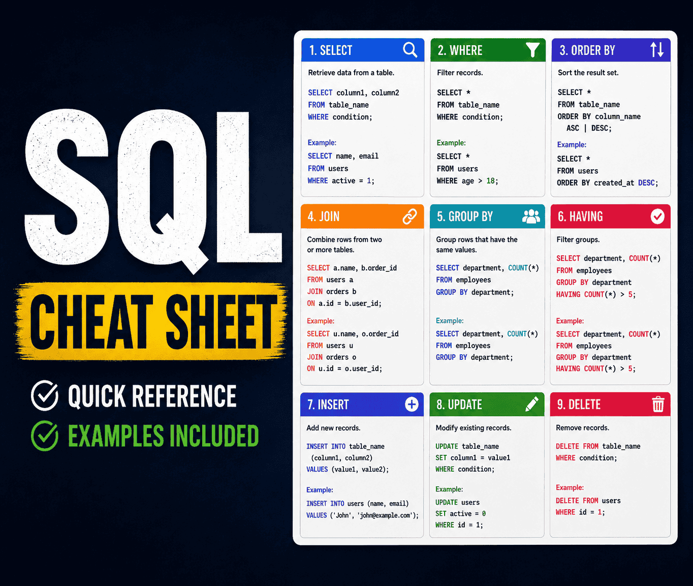
The Complete SQL Cheat Sheet 2026
Every SQL command, function, and pattern you need — from basic SELECT queries to advanced window functions, CTEs, indexes, and transactions. Clean, runnable examples for PostgreSQL, MySQL, and SQL Server.

Top 30 Most Asked System Design Interview Questions and Answers (2026 Edition)
Master the system design interview with this comprehensive guide covering load balancers, sharding, CAP theorem, and deep dives into 30 real-world design problems like WhatsApp, YouTube, and Uber.

Top 30 Node.js Interview Questions and Answers (2026 Edition)
Ace your next backend interview with this comprehensive guide covering the event loop, streams, clustering, async/await, Express.js, JWT authentication, caching, rate limiting, and graceful shutdown.
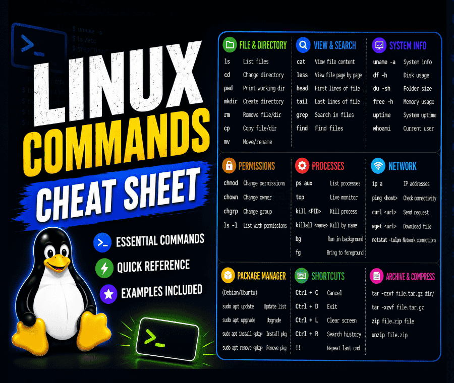
The Complete Linux Commands Cheat Sheet 2026
Every essential Linux command defined with clean, practical examples. Covers file navigation, system monitoring, user permissions, networking, package management, and shell scripting.